Betterment of Power System Performance Through Auxiliary Stabilizing Controller

(1)

© 2017, IRJET | Impact Factor value: 5.181 | ISO 9001:2008 Certified Journal

| Page 188

BETTERMENT OF

POWER

SYSTEM PERFORMANCE

THROUGH

AUXILIARY STABILIZING CONTROLLER

SHARAD CHANDRA RAJPOOT

1

_{, PRASHANT SINGH RAJPOOT}

2

_{, MUKESH KUMAR DEWANGAN}

3

1

_{Assistant professor (EE) G.E.C. Jagdalpur , Bastar, Chhattisgarh, India,}

2,3

_{Assistant professor (EE) L.C.I.T., Bilaspur, Chhattisgarh, India}

---***---Abstract- The response of the power system to a

disturbance may involve much of the equipment. For instance, a fault on a critical element followed by its isolation by protective relays will cause variations in power flows, network bus voltages, and machine rotor speeds; the voltage variations will actuate both generator and transmission network voltage regulators; the generator speed variations will actuate prime mover governors; and the voltage and frequency variations will affect the system loads to varying degrees depending on their individual characteristics. Further, devices used to protect individual equipment may respond to variations in system variables and cause tripping of the equipment, thereby weakening the system and possibly leading to system instability.

The operating characteristics of synchronous and induction machines are described by sets of differential equations. The number of differential equations required for a machine depends on the details needed to represent accurately the machine performance. The performance of the power system during the transient period can be obtained from the network performance equations. The performance equation using the bus frame of reference in either the impedance or admittance form has been used in transient stability calculations.

Index Terms- AC/DC power system, HVDC Line, power flows, network bus voltages , load flow analysis , stability analysis, power system stability.

1. INTRODUCTION1

Power system stability is the ability of an electric power system, for a given initial operating condition, to regain a state of operating equilibrium after being subjected to a physical disturbance, with most system variables bounded so that practically the entire system remains intact [2].

The power system is a highly nonlinear system that operates in a constantly changing environment; loads, generator

outputs and key operating parameters change continually. When subjected to a disturbance, the stability of the system depends on the initial operating condition as well as the nature of the disturbance. [10] Stability of an electric power system is thus a property of the system motion around an equilibrium set, i.e., the initial operating condition. In an equilibrium set, the various opposing forces that exist in the system are equal instantaneously or over a cycle.

HVDC Transmission has advantages over AC transmission in special situations [1]. The following are the types of applications for which HVDC transmission has been used:

1. Under water cables longer than about 30 km. AC transmission is impractical for such distances because of the high capacitance of the cable requiring intermediate compensation stations. 2. Asynchronous link between two AC systems where

AC ties would not be feasible because of system

Stability problems or a difference in nominal frequencies of the two systems.

1.1 OBJECTIVES

Stability is one of the important factor for the performance analysis of the any system. The essential objectives are-

1. To improve the system efficiency.

2. Mitigation of the losses to achieves maximum outcomes.

3. To reliable operation

4. Enhance the system active working life .

2. TRANSIENT STABILITY study for AC/DC SYSTEMS

2.1 overview

2.1.1 Power System Stability

(2)

© 2017, IRJET | Impact Factor value: 5.181 | ISO 9001:2008 Certified Journal

| Page 189

or loss of a large generator. A large disturbance may lead to

structural changes due to the isolation of the faulted elements. At an equilibrium set, a power system may be stable for a given (large) physical disturbance, and unstable for another. It is impractical and uneconomical to design power systems to be stable for every possible disturbance [2]. The design contingencies are selected on the basis that they have a reasonably high probability of occurrence. Hence, large-disturbance stability always refers to a specified disturbance scenario. Types of the power system stability are represents in the fig. no. 1

Fig.1 types of the stability

2.2 Transient Stability Studies

Transient stability studies provide information related to the capability of a power system to remain in synchronism during major disturbances resulting from either the loss of generating or transmission facilities, sudden or sustained load changes, or momentary faults. Specifically, these studies provide the changes in the voltages, currents, powers, speeds, and torques of the machines of the power system, as well as the changes in system voltages and power flows, during and immediately following a disturbance. The degree of stability of a power system is an important factor in the planning of new facilities. In order to provide the reliability required by the dependence on continuous electric service, it is necessary that power systems be designed to be stable under any conceivable disturbance.[10]

Fig.2 transient stability analysis [3]

A transient stability analysis is performed by combining a solution of the algebraic equations describing the network with a numerical solution of the differential equations. The solution of the network equations retains the identity of the system and thereby provides access to system voltages and currents during the transient period [5].

2.3 Analytical Elimination

To illustrate the procedure, the analytical elimination is carried out in detail for some representative modes. It is sufficient to find Pd and Sd at each converter, since Qd then

can be computed. The partial derivatives for all modes.

Control Mode A:

[αr γi Vdi Pdi] (1)

Since both the voltage and power at the inverter are specified, the direct current can be computed, and Pdr can

then be found by combining Pdr = Pdi + Rd Id2

(2) If we combine

2

3

cos

di d c d

dr

r

P R X I

S k 



 

_  _

 



k

_



P

_di

 

P Q

_l _l



(3) Analogously, for Sdi:









cos

di di l di l

i k

S  _ P Q k P Q

(3)

© 2017, IRJET | Impact Factor value: 5.181 | ISO 9001:2008 Certified Journal

| Page 190

Thus, all real and reactive powers consumed by the

converters can be precomputed, and including the dc-link in the power flow is trivial for this control mode. The same is true for any specification of the form [αr γi x1 x2], where x1

and x2 are any two variables of [Pdr Pdi Vdr Vdi Id]. The fact

that the real and reactive powers can be precomputed for this case is well known.

Control Mode B:

[αr γi Vdi Pdi] (5)

This mode occurs e.g. if the tap changer at the rectifier hits a limit in control mode A under current control in the rectifier. Since Pdi and Vdi are specified, Id, Vdr, Pdr and Sdi computed as

for mode A. Since αr is specified, Sdr is computed with (3)

instead of (4).

3 2

dr

tr tr r d dr

tr S

V V k a I S

V      _ _  _ _ (6) 2 dr dr tr tr dr Q S V V Q  _  (7)

The formulas for mode BI are essentially identical; the only

difference is that Pdi, rather than Id, is computed with (5). In

general, when two of the variables of [Pdr Pdi Vdr Vdi Id] are

specified, the other three can be computed from (3)-(5).

Control Mode C:

[αr γi ai Pdi]

These specifications are valid e.g. if the tap changer at the inverter hits a limit in mode A under current control in the rectifier. Combining (2) and (5) gives

2

3 2

3 cos

di i ti i d c d

P

a V



I

X I







(8) If we solve for Id, we obtain





2

1 1 2

d ti ti di

I



c V



c V



c P

(9)





2 1 1 ₂ 1 2 d ti ti ti di

I

c V

c

V

_{c V}

_{c P}



_{ }



_

(10) where 1

cos

2

i i c

a

c

X





(11) 2

3

_c

c

X





(12)

Define ∂Ii as

ti d i d ti

V

I

V



 



(13)

Since Pdi is specified, both its partials are zero. Pdr is given by

(4),and its partial derivatives by:

0

dr tr tr

P

V







(14) 2

2

dr ti d

ti d d l i

ti d ti

P

V

I

V

R I

P I

V

I

V



_



_

_



(15)

Since

a

_iis specified, Sdi is computed with (7), and the partial

derivatives of Qdi are given by

0

di tr tr

Q

V



_



(16)





2

1

di di ti i ti di

Q

S

V

I

V

Q



_

_{ }



(17)

Qdr and its partial derivatives are computed from (5)





2

dr

ti i l l

ti

S

V

I k

P

Q

V





_{ }

_



(18)

0

dr tr tr

Q

V







(19)





2

dr i

ti dr l l l dr

ti dr

Q

I

V

k S

Q

P

PP

V

Q





_

_{ }

_

_

_







(20)

Other Modes

The partial derivatives for the other control modes can be derived analogously; if the tap changer controlling the control angle is specified (modes B, D, F, G), only the reactive power at that converter will depend on corresponding AC voltage.

If the tap changer controlling the direct voltage is specified (modes C, D, E, G), all the real and reactive powers will depend on the AC voltage at that terminal. Equations (17) are used to find the direct current for constant power control.

2.3.1 Representation of Loads

(4)

© 2017, IRJET | Impact Factor value: 5.181 | ISO 9001:2008 Certified Journal

| Page 191

either static impedance or admittance to ground, constant

real and reactive power, or a combination of these representations. The parameters associated with static impedance and constant current representations are obtained from the scheduled bus loads and the bus voltages calculated from a load flow solution for the power system prior to a disturbance [5]. The initial value of the current for a constant current representation is obtained from

*

lp lp

po

p

P

jQ

I

E





(21)

The static admittance Ypo used to represent the load at bus P,

can be obtained from

po po

p

I

Y

E



(22)

where Ep is the calculated bus voltage, Plp and Qlp are the

scheduled bus loads. Diagonal elements of Admittance matrix (Y – Bus) corresponding to the load bus are modified using the Ypo.

2.3.2 Representation of HVDC Systems

Each DC system tends to have unique characteristics tailored to meet the specific needs of its application. Therefore, standard models of fixed structures have not been developed for representation of DC systems in stability studies [1].

a) Converter model

i) Simplified model

Here valve switching is neglected and the converter is represented by the average DC voltage equation. This model is similar to that used in power flow analysis. The transformer tap is assumed to be constant as the tap changer dynamics are very slow [7]. This model is inaccurate during severe disturbances. It cannot handle commutation failures and cannot predict the converter behavior during unsymmetrical faults.

ii) Detailed model

Here, the valve switching is incorporated and the model is free from the drawbacks associated with the simplified model. However the transient simulation of converter now requires integration step size as small as 50 – 100 μs. This implies heavy computation burden, so it is used only for short duration (say 0.2 sec) immediately after the disturbance.

b) Converter controller models

i) Response type model

The dynamics of the CEA and CC are neglected and only the steady – state controller characteristics are represented. The main feature of this type of controller model is that the configuration and the parameters of the controller are assumed to designed at a later stage basing on the requirement.

ii) Detailed representation

It requires the analysis of actual control circuitry and the establishment of a dynamic equivalent with a frequency response which matches the actual controller response. This is used along with the detailed converter model.

c) DC network model

i) Resistive network

Here DC network is represented as resistive network ignoring energy storage elements. This approach is valid when DC lines are short and or for back to back HVDC links and smoothing reactors are of moderate size.

ii) Transfer function representation

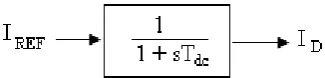
For a two terminal DC link with the response type controller, an alternative representation of the DC network is to use a transfer function (Fig. 3) instead of a resistance. In this case, the time constant Tdc represents the delay in establishing the

DC current after a step change in the order is given.

Fig. 3 Transfer Function Model

iii) Dynamic representation

[image:4.595.353.516.512.551.2]

As the frequency bandwidth of the response model considered in the transient stability studies is modest, it is adequate to represent the dc network by a simple equivalent circuit of the type shown in figure no 4 Even here, the shunt branches may be neglected.

(5)

© 2017, IRJET | Impact Factor value: 5.181 | ISO 9001:2008 Certified Journal

| Page 192

2.3.3 Runge-Kutta method

In the application of the Runge-Kutta fourth-order approximation, the changes in the internal voltage angles and machine speeds, again for the simplified machine representation, are determined from

 





 





1 2 3 4

1

2

6

1

2

6

i i i i

i t t

i i i i

i t t

k

l



















(23)

i=1,2,…,no. of generators.

The k’s and l’s are the changes in



i and



i respectively,

obtained using derivatives evaluated at predetermined points. For this procedure the network equations are to be solved four times.

3. ENHANCEMENT OF AC SYSTEM PERFORMANCE HVDC CONTROLS

In a DC transmission system, the basic controlled quantity is the direct current, controlled by the action of the rectifier with the direct voltage maintained by the inverter. A DC link controlled in this manner buffers one AC system from disturbances on the other. However, it does not allow the flow of synchronizing power which assists in maintaining stability of AC systems. The converters in effect appear to the AC systems as frequency-insensitive loads and this may contribute to negative damping of system swings [1]. Further, the DC links may contribute to voltage collapse during swings by drawing excessive reactive power.

The above signals work satisfactorily for the single machine system case. However, in the case of multi-machine system it may be necessary to employ control signals derived from relative angle deviation, speed deviation and acceleration and different combinations of these signals. Apart from linear controllers, (like P, PI and PID controllers) Fuzzy logic controllers can also be employed which are known to give better performance. The output of Fuzzy Logic Controller is utilized to modulate the power order of the DC control, which in turn modulates the DC power.

3.1 Proposed Work

In this work, the advantage of fast HVDC power modulation is utilized to improve the stability of the system with different types of controllers and control signals.

3.1.1 Case 1

A multi machine system is considered with a HVDC link having a Proportional Integral current controller. The auxiliary controller is a constant gain controller which is given with different control signals from the AC system. The control signals are derived from relative generator angles, relative speed variations and accelerations of different generators.

3.1.2 System Data

 Generator :

Pg=2.0 pu H=4.0 pu Xd=0.2 pu D=0.02

F=50Hz

 AC transmission lines: Xeq = 0.16 pu

 Transformer: Xt=0.24 pu

 DC link:

K1=0.1 K2=0.2 Tw=0.04

Ld=0.02 Rd=0.05 Xc=0.124

 Initial conditions δ=0.4534 Δw =0 Id=0.8865

Alfa=0.310 Vdi=0.987

4 CONTROL STRATEGIES

4.1 Introduction

The stability analysis is carried out on a single machine system and on a multi machine system, considering different controllers and control signals. The details of the controllers and the control signals used along with the results obtained from different case studies, indicating the stability of the system, are presented in this chapter.

4.2 Single Machine System Analysis

4.2.1 Auxiliary Stabilizing Controller

(6)

| Page 193

Fig. 4: Type - 0 Controller

4.2.2 Case B: Line Outage

One of the parallel AC lines is given outage, here the two ac lines are assumed to be similar. Therefore this disturbance can be reflected by varying the value of Xeq, which represents

the equivalent reactance of both the lines. Here, once again the different signals are utilized for stability improvement. The plots of generator angles for different stabilizing signals are shown in figures 5 – 10.

0 2 4 6 8 10 12

0.639 0.64 0.641 0.642 0.643 0.644 0.645 0.646 0.647 0.648 0.649

time(sec)

d

e

l(

ra

d

)

[image:6.595.42.280.104.224.2]

del

Fig. 5: Plot of generator angle without any external control signal.

0 2 4 6 8 10 12

0.6425 0.643 0.6435 0.644 0.6445 0.645 0.6455 0.646 0.6465 0.647

time(sec)

d

e

l(

ra

d

)

[image:6.595.320.537.109.276.2]

del

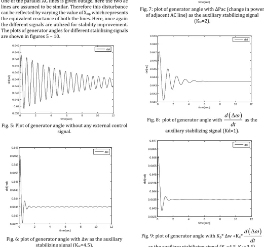
Fig. 6: plot of generator angle with Δw as the auxiliary stabilizing signal (Kw=4.5).

0 2 4 6 8 10 12 14 16 18 20

0.6425 0.643 0.6435 0.644 0.6445 0.645 0.6455 0.646 0.6465 0.647

time(sec)

d

e

l(

ra

d

)

del

Fig. 7: plot of generator angle with ΔPac (change in power of adjacent AC line) as the auxiliary stabilizing signal

(Kw=2).

0 2 4 6 8 10 12

0.641 0.642 0.643 0.644 0.645 0.646 0.647 0.648 0.649

time(sec)

d

e

l(

ra

d

)

[image:6.595.34.556.271.759.2]

del

Fig. 8: plot of generator angle with

d

 

dt





as the

auxiliary stabilizing signal (Kd=1).

0 2 4 6 8 10 12

0.6425 0.643 0.6435 0.644 0.6445 0.645 0.6455 0.646 0.6465 0.647

time(sec)

d

e

l(

ra

d

)

del

Fig. 9: plot of generator angle with Kp* Δw +Kd*

 

d

dt





[image:6.595.50.263.357.511.2]

(7)

| Page 194

0 2 4 6 8 10 12

0.6425 0.643 0.6435 0.644 0.6445 0.645 0.6455 0.646 0.6465 0.647

time(sec)

d

e

l(

ra

d

)

[image:7.595.44.280.103.300.2]

del

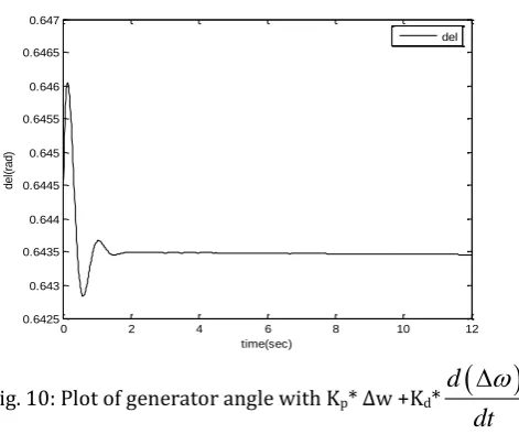
Fig. 10: Plot of generator angle with Kp* Δw +Kd*

 

d

dt





+KiΔδ as the auxiliary stabilizing signal (Kp=1.4, Kd =0.12,

Ki=0.0005).

10. CONCLUSION

For a parallel line outage, the variation in power, in the other parallel line, when used as the control signal, gives better performance as shown in figures 5 to 10.

Stability of the system must be in desired limit for the efficient & proper performance of it. It can be analyze with and without changes in the input control signal, which are express in the fig. 5 to 10. It is mostly influenced by the power angle. This can be controlled with the variation in the speed of the synchronous generator. For the single machine system stability can be change with the help of input control signals. Stability of the system will responsible for the enhancing the reliability and performance of the system. This will influenced the efficiency of the power system.

SCOPE OF FUTURE WORK

By varying the value of the Kp KD & KW ,the out put changes.

This are observed by the analysis of the waveform .By using fuzzy logic the gains of the control signal, specified in the last chapter, are adjusted in every sampling interval in accordance to a set of linguistic control rules and in conjunction. This feature is desirable because as the operating conditions of a system begin to change, deterioration in performance will result if a fixed gain controller is applied.

11.REFERENCES

1. P. Kundur, “Power System Stability and Control”, McGraw- Hill, Inc., 1994.

2. Prabha Kundur, John Paserba, “Definition and Classification of Power System Stability”, IEEE

Trans. on Power Systems., Vol. 19, No. 2, pp 1387- 1401, May 2004.

3. A.Panosyan, B. R. Oswald, “Modified Newton- Raphson Load Flow Analysis for Integrated AC/DC Power Systems”,

4. T. Smed, G. Anderson, “A New Approach to AC/DC Power Flow”, IEEE Trans. on Power Systems., Vol. 6, No. 3, pp 1238- 1244, Aug. 1991.

5. Stagg and El- Abiad, “Computer Methods in Power System Analysis”, International Student Edition, McGraw- Hill, Book Company, 1968.

6. Jos Arrillaga and Bruce Smith, “AC- DC Power System Analysis”, The Institution of Electrical Engineers, 1998.

7. K. R. Padiyar, “HVDC Power Transmission Systems”, New Age International (P) Ltd., 2004.

8. “IEEE Guide for Planning DC Links Terminating at AC Locations Having Low Short-Circuit Capacities”, The Institute of Electrical and Electronics Engineers, Inc., 1997.

9. Garng M. Huang, Vikram Krishnaswamy, “HVDC Controls for Power System Stability”, IEEE Power Engineering Society, pp 597- 602, 2002.

10. Sharad Chandra Rajpoot, Prashant Singh Rajpoot and Durga Sharma,”_{Power system Stability}

Improvement using Fact Devices”,_{International}

Journal of Science Engineering and Technology research ISSN 2319-8885 Vol.03, Issue. 11,June-2014,Pages:2374-2379.

11. Sharad Chandra Rajpoot, Prashant singh Rajpoot and Durga Sharma,“Summarization of Loss Minimization Using FACTS in Deregulated Power System”, International Journal of Science Engineering and Technology research ISSN 2319-8885 Vol.03, Issue.05,April & May-2014,Pages:0774-0778.

12. Sharad Chandra Rajpoot, Prashant Singh Rajpoot and Durga Sharma, “Voltage Sag Mitigation in Distribution Line using DSTATCOM” International Journal of ScienceEngineering and Technology research ISSN 2319-8885 Vol.03, Issue.11, April June-2014, Pages: 2351-2354.

(8)

| Page 195

research ISSN 2319-8885 Vol.03, Issue.08,

May-2014, Pages: 1343-1348.

14. Sharad Chandra Rajpoot, Prashant Singh Rajpoot and Durga Sharma, “A typical PLC Application in Automation”, International Journal of Engineering research and TechnologyISSN 2278-0181 Vol.03, Issue.6, June-2014.

15. Iba K. (1994) ‘Reactive power optimization by genetic algorithms’, IEEE Trans on power systems, May, Vol.9, No.2, pp.685-692.

16. Sharad Chandra Rajpoot, Prashant Singh Rajpoot and Durga Sharma,“21st_{century modern technology}

of reliable billing system by using smart card based energy meter”,International Journal of Science Engineering and Technology research, ISSN 2319-8885 Vol.03,Issue.05 ,April & May-2014,Pages:0840-0844.

17. Prashant singh Rajpoot , Sharad Chandra Rajpoot and Durga Sharma,“wireless power transfer due to strongly coupled magnetic resonance”_{, international}