Modeling Preparative Chromatographic Separation of Heavy Rare Earth Elements and Optimization of Thulium Purification

http://dx.doi.org/10.4236/ampc.2015.55016

How to cite this paper: Max-Hansen, M., et al. (2015) Modeling Preparative Chromatographic Separation of Heavy Rare Earth Elements and Optimization of Thulium Purification. Advances in Materials Physics and Chemistry, 5, 151-160.

http://dx.doi.org/10.4236/ampc.2015.55016

Modeling Preparative Chromatographic

Separation of Heavy Rare Earth Elements

and Optimization of Thulium Purification

Mark Max-Hansen, Hans-Kristian Knutson, Christian Jönsson, Marcus Degerman,

Bernt Nilsson

Department of Chemical Engineering, Lund University, Lund, Sweden Email: *[email protected]

Received 28 January 2015; accepted 26 April 2015; published 29 April 2015

Copyright © 2015 by authors and Scientific Research Publishing Inc.

This work is licensed under the Creative Commons Attribution International License (CC BY). http://creativecommons.org/licenses/by/4.0/

Abstract

Rare Earth Elements are in growing demand globally. This paper presents a case study of applied mathematical modeling and multi objective optimization to optimize the separation of heavy Rare Earth Elements, Terbium-Lutetium, by means of preparative solid phase extraction chromatogra-phy, which means that an extraction ligand, HDEHP, is immobilized on a C18 silica phase, and ni-tric acid is used as an eluent. An ICP-MS was used for online detection of the Rare Earths. A me-thodology for calibration and optimization is presented, and applied to an industrially relevant mixture. Results show that Thulium is produced at 99% purity, with a productivity of 0.2 - 0.5 kg Tm per m3 _{stationary phase and second, with Yields from 74% to 99%.}

Keywords

Rare Earth Elements, Chromatography, Model Calibration, Optimization, Multi-Objective, HDEHP

1. Introduction

The Rare Earth Elements (REEs) are Scandium and Yttrium and the members of the Lanthanide group in the periodic table. Many of these metals are used in batteries, lasers, capacitors, superconductors [1], which make the purification process demanding through high purity requirements in some of these applications. Current in-dustrial separation methods include liquid-liquid extraction, selective oxidation/reduction, and ion exchange chromatography [2]-[5]. Extraction chromatography is commonly used for analytical purposes [1] [6]-[9].

The REEs are of growing economic importance, with China limiting the export quotas [10] [11], which

creates a demand for alternative sources, and alternative purification processes, as the currently dominating liquid- liquid extraction uses high quantities of organic compounds for the separation. Solid phase extraction or extrac-tion chromatography uses smaller amounts of organic chemicals than liquid-liquid extracextrac-tion. This is why solid phase extraction could be one of the alternative purification processes.

This work is a continuation of the work presented in [12]-[14] where a mixture of the elements from Neody-mium to Gadolinium was used in modeling and optimization of a chromatographic step, and also in experimen-tal optimization. In the present work a mixture of all REEs except Scandium was separated on a modified col-umn that operates in a solid phase extraction mode, meaning that the extractant is immobilized as a ligand in the column. To find the optimal operating conditions for the separation, a Dispersive-Equilibrium model was con-structed, based on Langmuirian type binding with mobile phase modulator. The parameters for the model were calibrated from isocratic and gradient experiments. The optimal operating points were found by applying an op-timization algorithm on the calibrated model and performance functions. In addition to this one of optimal oper-ating points was verified experimentally.

2. Theory

To design and optimize the chromatographic system, a performance function is required. This in turn depends on a mathematical formulation of the physical chromatography system. This mathematical formulation requires retention parameters, mass transfer parameters and column capacity to be calibrated. To reduce the complexity of the calibration, only the retention parameters are calibrated with a less computationally expensive model, i.e. the retention volume model. These retention parameters are then used as a starting guess in the more advanced model of the chromatography column, which takes dispersion and mass transfer effects into account as well as the retention data. For the optimization, Productivity and Yield were selected as performance functions, subject to a Purity constraint.

2.1. The Retention Volume Model

The retention volume model is an ideal model, which can be seen as a simplified version of the film mass trans-fer model, presented in 2.2, that includes the isocratic modifier concentration effect on the retention volume:

(

)

0 1

R R c P D

V =V + −ε ⋅ε ⋅K ⋅H (1)

where VR is the retention volume, VR0 is the retention volume under non-binding conditions, εC is the column porosity, εP is the particle porosity, KD is the exclusion factor and H is the Henry constant [15]:

0 modifier

H=H ⋅s−ν (2)

where H0 is the Henry constant when the modifier concentration is unity, smodifier is the modifier concentration (mol/m3), ν is the stochiometric coefficient. This expression is valid only when the loaded amount is much smaller than the total adsorption capacity.

2.2. The Dispersive-Equilibrium Model

The model including mass transfer and non-linear effects is a Dispersive-Equilibrium model using Langmuir type binding with mobile phase modifier, consisting of a dispersive-equilibrium description of the mobile phase with all mass transfer effects lumped in the dispersion, and Langmuir equilibrium adsorption for the solid phase

[16]. For component i, its liquid-phase concentration in the column is described by the following equation:

2

2

1

i i i i

AX app

T

c c c q

D v

t ⋅ x x ε ⋅ t

∂ ∂ ∂ ∂

= − −

∂ ∂ ∂ ∂ (3)

(

)

0 app

i

i inlet i

AX x

v c

c c

x D ₌

∂

= −

∂ (4)

where cinlet,i is the concentration of component i at the inlet. The concentration of species i at x = 0 may be lower than the inlet concentration due to dispersion. The other boundary condition is at the outlet of the column, at x = L, and is a von Neumann condition:

0 i x L c x ₌ ∂ =

∂ (5)

The concentration of species i adsorbed on the stationary phase is described by the following equation, which is a mobile phase modified version of the Langmuir adsorption description [21]:

0

max,

0 1 i

i i

i q

H s c q

q

ν

−  

= ⋅ ⋅ ⋅ −_ _−



∑

where H0 is the Henry constant, s is the modifier concentration, ν is the stochiometric constant, qmax,i is the maximum adsorption capacity for component i. This equation must at equilibrium satisfy the adsorption equili-brium isotherm, which means that the parenthesis must be 0 at equiliequili-brium.

The flow rate dependence of the apparent dispersion, including mass transfer resistance and kinetics, is ap-proximated with a second degree polynomial. This comes from the Knox equation [17]:

1 3

app p app p

app p

B

h Av d Cv d

v d

= + + (7)

where h is the reduced plate height, vapp is the apparent velocity, dp is the particle diameter. A, B and C are con-stants coming from flow structure and non equilibrium effects. The apparent axial dispersion can then be de-scribed as: 2 AX app h D v

= (8)

where DAX is the apparent dispersion coefficient. Combining equations 7 and 8 give:

4 2 3

1

2

AX app app

D = ⋅_B+Av +Cv _

  (9)

Estimating the apparent dispersion with a second degree polynomial gives a small error in the second term, however this is acceptable with current model precision.

2.3. Optimization

The target component for the optimization is Thulium, as producing pure Thulium would produce pure Ytter-bium also, and then both of the major components have been purified, see Figure 4 and Figure 5. The rest of the REEs are considered impurities. The optimal performance of the separation system depends on the technical and economic constraints and incentives that are placed upon this system. Common performance attributes used are Productivity, Yield, Purity and Specific Productivity. In this work, Productivity, presented in Equation (10) and Yield, presented in Equation (11) are used as performance functions, while the Purity is used as a constraint. The productivity can be calculated from:

,2 ,1 d cut cut t outlet t cycle col

F c t

Pr t V ⋅ = ⋅

∫

,2

,1

0

d d

cut cut load

t

outlet t

t

feed

F c t

Y

F c t

⋅ =

⋅

∫

∫

In this case tload is the time at the end of the loading(s), cfeed is the concentration in the feed (mol/m 3

).

When two competing objectives, in this case productivity and yield are competing, the result will be a Pareto front, which means that for a given optimal point on the front, increasing one objective must decrease the other

[18]-[20].

3. Materials and Methods

3.1. Materials

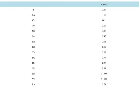
The experiments were performed on an Agilent 1260 Bio-Inert HPLC system, consisting of two Agilent 1260 Bio-Inert Quaternary pumps, one Agilent Bio-Inert 1260 Autosampler and one Agilent 1260 Bio-Inert UV/Vis detector connected to an Agilent 7700 ICP-MS for detection of the rare earths. The column preparation was performed using a GE Healthcare ÄKTA Purifier 100. The individual rare earths were acquired from Merck at 1 g/L in nitric acid. The concentrated nitric acid of HPLC grade was acquired from Merck. The columns used were Kromasil C18, 100 Å, 16µm columns with immobilized HDEHP acting as ligand. HDEHP was acquired from Merck. Methanol was acquired from Merck. To be able to do higher flow rate experiments, an extra iso-cratic pump was added to the system after the column, and used to feed the ICP-MS with a constant flow of 1 ml/min, the rest going to waste or collection. The heavy mixture of rare earths used in the Thulium optimization was mixed to mimic an industrially relevant REE-stream, with a composition as described inTable 1.

Column Preparation

The column was modified by passing a mixture of 22 mM HDEHP in 65% (v/v) Methanol-water, using the conductivity meter of the ÄKTA to determine the breakthrough volume, and thereby the ligand concentration of 345 mol/m3 column volume. As the ligand forms dimers, the concentration of sites was 172.5 mol/m3 column volume.

Table 1. Composition of heavy mixture, 336 g/L, 14 M HNO3.

% (wt)

Y 0.67

La 1.2

Ce 0.1

Pr 0.09

Nd 0.13

Sm 0.42

Eu 0.06

Gd 1.59

Tb 0.13

Dy 0.74

Ho 4.23

Er 6.54

Tm 11.99

Yb 71.89

3.2. Methods

Isocratic experiments at 16 compositions of the mobile phase were performed to get retention volumes for all components, gradient experiments at different flow rates were performed to get peak broadening from mass transfer and kinetics.

3.2.1. Experimental Design for Calibration

16 isocratic experiments, 0.35 to 4.9 M nitric acid were performed, with 3 replicates on all experimental points. The experiments were performed at 0.35, 0.53, 0.56, 0.60, 0.63, 0.67, 0.70, 1.05, 1.40, 1.75, 2.10, 2.8, 3.50, 4.20 and 4.90 M nitric acid concentration, using the quaternary pump to create the isocratic eluent.

No overloading experiments were performed, as the column capacity had been decided during the preparation of the column.

3.2.2. Chromatography Method

The chromatographic experiments performed, consisted of four consecutive steps; loading, isocratic elution, Cleaning in Place (CIP), and reequilibration.

The injected amount during loading was 10 µl of a mixture containing 0.0357 g/L of each of the lanthanides, plus yttrium. This was well within the linear range of the isotherm, so any competitive effects could be neg- lected. After loading, a prepared eluent of a predetermined concentration was passed through the column for 120 minutes, this was due to a limitation of the ICP-MS software, after elution a CIP at 7M nitric acid was per-formed. After the CIP the system was reequilibrated with water. All experiments were performed with three rep-licates.

3.2.3. Validation Experiment Chromatography Method

For the validation experiment, the experimental setup was modified so that it no longer had the post column pump. This decreased the post column dispersion. The validation experiment was adjusted somewhat from the very aggressive points on the Pareto front, to a longer gradient and with a lower flow rate. The validation expe-riment consisted of five consecutive steps: loading, wash, gradient elution, CIP and reequilibration. The injected amount during loading was 200 µl heavy mixture, diluted to 33.6 g/L with deionized water, then a 4.5 ml wash with deionized water, followed by a 17 ml gradient from 0 to 7 M nitric acid. Then 4 ml CIP at 7 M nitric acid, followed by 10 ml reequilibration with deionized water.

3.2.4. Simulation Method

The chromatography model was discretized in the axial direction, to turn the partial differential equation into a system of Ordinary Differential Equations (ODE) and Algebraic equations, Differential Algebraic Equation (DAE). The discretization used a 2 point backward finite difference scheme for the flow, and a 3 point central finite difference scheme for the dispersion. The assembled DAE system was solved with MATLAB ODE/DAE solver ode 15 s, which solves stiff DAEs. Discretization and Simulation is handled by the Preparative Chroma-tography Simulator, PCS, developed at the Department of Chemical Engineering, Lund University [21]. In order to reduce the size of the computational problem for the optimization, all components lighter than Gadolinium were lumped together and added to the mass of Gadolinium, this is done, as in the worst case perspective of se-parating Thulium from the heavy mixture, they would act as Gadolinium, where they would pass more readily through the column in reality.

3.2.5. Calibration Method

First the Henry constant and the stochiometric coefficient were calculated from the slope and intercept of the logarithm of the modified retention volume, versus the logarithm of the modifier concentration. These were then used for the inverse method, i.e. minimizing the least squares error for the normalized detector response and the normalized simulated chromatograms, where the mass transfer effects were fitted, using a Nelder-Mead simplex algorithm. The maximum binding capacity of the columns was decided during preparation of the columns, and based on the HDEHP concentration in the backbone.

3.2.6. Optimization Method

Dif-ferential Evolution (DE) algorithm and parallel computations in a cluster environment [13]. For the optimization, four decision variables were chosen, load volume, gradient length, CIP length and flow rate.

4. Results

The modified columns had some known characteristics, such as the porosities, εc = 0.6, εp= 0.4, and the maxi-mum binding capacities, which were decided during the impregnation of the column, and calculated from equa-tion 12:

max,i i

q λ

ν

= (12)

where λ is 172.5 (mol/m3 column), and νi is the stochiometric constant for component i.

4.1. Model Calibration

The Henry constants and characteristic charges, presented inTable 2, were calculated from the retention volume experiments presented in Figure1. There is a wide span in retention data for the replicates, as can be seen in Figure 1. This is probably a result of non-isocratic and inexact mixing of the eluent as a result of the rotating inlet valve combined with the non-ideal mixing properties of water and nitric acid.

Figure 1. Retention data for the experiments, with regressed lines. There is a wide span in retention data for the replicates, as can be seen in the figure above.

Table 2. The fitted stochiometric coefficients and Henry constants.

Component ν H qmax

Yttrium 2.18 22.96 79

Terbium 2.20 21.07 78

Dysprosium 1.96 20.24 88

Holmium 2.12 21.89 81

Erbium 2.34 24.49 73

Thulium 2.19 24.29 78

Ytterbium 2.25 25.60 77

Lutetium 2.64 29.47 65

6.5 7 7.5 8 8.5 9

4 4.5 5 5.5 6 6.5 7 7.5 8 8.5 9

log C_mod

log (

Vr

- V

r0

)

log (V_r - V_r0 ) versus log c_mod

4.2. The Flow Rate Experiments

To calibrate the mass transfer effects, flow rate experiments were performed at 1, 1.25, 1.5, 1.75, 2, 2.5 and 3 ml/min, the normalized detector response was used against a normalized simulated response from the PCS, and parameters fitted by a least squares approach. The experimental and model results are presented in Figure 2, with model parameters for the axial dispersion as in Equation (9), with the terms: A = 1.05 × 10−8, B = 1.00 × 10−8 and C = 0.9936 × 10−8.

4.3. Optimization

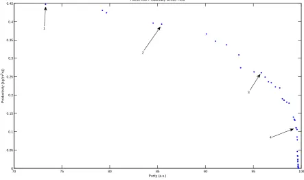
The multi-objective optimization was performed using Productivity and Yield, see Equations (10) and (11), as objective functions. The optimization output is a the Pareto front, presented in Figure 3, which gives the system

Figure 2. Model response and experimental response for dysprosium at different flow rates. There is a reasonably good fit, and using a least squares approach to model calibration will result in wider peaks where there is variation in the experiments.

Figure 3. Pareto front Productivity versus Yield, selected Pareto points correspond to chromatograms inFigure 4.

200 400 600 800 1000 1200 1400

-0.005 0 0.005 0.01 0.015 0.02 0.025

70 75 80 85 90 95 100

0 0.05 0.1 0.15 0.2 0.25 0.3 0.35 0.4 0.45

Purity (a.u.)

P

roduc

ti

v

it

y

(

k

g/

(m

3s⋅

))

Pareto front Productivity versus Yield

1

2

3

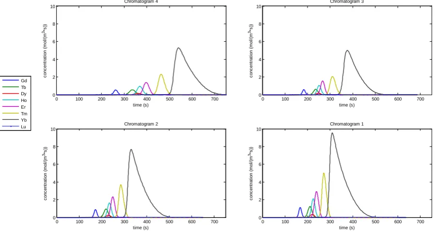
performance for different operating points, comparing in this case Productivity and Yield, under a 99% Purity constraint for the Thulium. Figure 3shows that the Pareto front is much denser in the high yield region, than it is in the high productivity region. This is to be expected, as high yields are relatively easy to achieve by keeping the loading volume small, and the gradient slope flat. The selected points in Figure 3are presented in Figure 4, with their decision variables presented inTable 3.

All of the operating points are under overloaded conditions, as can be seen inFigure 4, with a decreasing de-gree of overloading as we move from high productivity in chromatogram 1 to high yield in chromatogram 4. The curvature of the Pareto front is a result of peak overlapping, so that in chromatogram 4, the Thulium peak is slightly contaminated on the back side by Ytterbium but base line separated at the front, then going to chroma-togram three, where the Thulium peak is contaminated more by Ytterbium at the back side, and starting to see Erbium at the front side. Chromatogram 2 shows even more Ytterbium in the back side of the peak, and a bit of Erbium at the front side as well. In chromatogram 1, the Erbium and Ytterbium peaks almost meet underneath the Thulium peak.

4.4. Validation

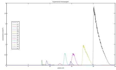
As described in 3.2.2, the validation experiment was performed at a slightly less aggressive operating point than max (Prod * Yield), with a longer gradient and a flow rate of 1 ml/min. The chromatogram from the validation experiment, presented in Figure 5 shows that base line separation on the front side of the Thulium peak is poss-ible, with a small overlap at the back side, while both Thulium and Ytterbium show overloaded conditions. This

Figure 4. Selected chromatograms from the Pareto front. All chromatograms are overloaded, with decreasing degree from chromatogram 1 to chromatogram 4.

Table 3. The chromatograms fromFigure 3 andFigure 4, with their decision variable values and Productivity and Yield values.

Prod (kg/m3_{·s) Yield (%wt) Load (ml) Gradient length (ml) Flow rate(ml/min)}

Chromatogram 1 0.181 98.5 0.0684 7.70 1.26

Chromatogram 2 0.263 95.1 0.0672 5.17 1.55

Chromatogram 3 0.396 84.5 0.110 5.62 1.68

Chromatogram 4 0.447 73.3 0.140 5.66 1.73

0 100 200 300 400 500 600 700

0 2 4 6 8 10 time (s) c onc ent rat ion ( m ol /( m 3*s )) Chromatogram 4

0 100 200 300 400 500 600 700

0 2 4 6 8 10 time (s) c onc ent rat ion ( m ol /( m 3*s )) Chromatogram 3

0 100 200 300 400 500 600 700

0 2 4 6 8 10 time (s) c onc ent rat ion ( m ol /( m 3*s )) Chromatogram 2

0 100 200 300 400 500 600 700

Figure 5. Experimental chromatogram. This slightly overloaded chromatogram shows base line separation at the front side of the Thulium peak, and a slight overlap on the back side of the peak. This means high purity and high yield.

chromatogram has a calculated Productivity of 0.20 kg Thulium per cubic meter of column volume and second, with a Yield above 95%. The reason that the peaks are a lot sharper in the validation chromatogram than the si-mulated peaks, is that the post column pump was removed, which leads to much less post column dispersion.

5. Conclusion

Using the inverse method to fit retention data and kinetics at the same time for a system with 15 components is very hard, for this reason, performing isocratic experiments to determine the isotherm parameters, and using the inverse method for the mass transfer effects proved to be an easier path to follow. The model predicts prepara-tive loads under gradient elution well, and therefore is applicable in optimizations of the separation system, for a wide range of mixtures and performance criterion. The performance of the system showed a Productivity range for Thulium from 0.18 kg/(m3∙s) to 0.45 kg/(m3∙s) at Yields of 98.5% to 73.3%.

References

[1] Verma, S.P. and Santoyo, E. (2007) High-Performance Liquid and Ion Chromatography: Separation and Quantification Analytical Techniques for Rare Earth Elements. Geostandards and Geoanalytical Research, 31, 161-184.

[2] Pierce, T.B. and Hobbs, R.S. (1963) The Separation of the Rare Earths by Partition Chromatography with Reversed Phases: Part 1. Behavior of Column Material. J Chrom A, 12, 74-80.

[3] Russell, R.G. and Pearce, D.W. (1943) Fractionation of the Rare Earths by Zeolite Action. Journal of the American Chemical Society, 65, 595-600. http://dx.doi.org/10.1021/ja01244a029

[4] Lister, B.A. and Smith, M.L. (1948) The Fractionation of Cerium (III) and Neodymium Mixtures on an Ion-Exchange Column. Journal of the Chemical Society, 1272-1275. http://dx.doi.org/10.1039/jr9480001272

[5] Choppin, G.R. and Silva, R.J. (1956) Separation of the Lanthanides by Ion Exchange with Alpha-Hydroxy Isobutyric Acid. Journal of Inorganic and Nuclear Chemistry, 3, 153-154. http://dx.doi.org/10.1016/0022-1902(56)80076-6

[6] Harris, D.H. and Tompkins, E.R. (1947) Ion-Exchange as a Separation Method; Separations of Several Rare Earths of the Cerium Group (La, Ce, Pr and Nd). Journal of the American Chemical Society, 69, 2792-2800.

http://dx.doi.org/10.1021/ja01203a061

0 5 10 15 20 25

0 0.5 1 1.5 2 2.5 3

volume (ml)

c

onc

ent

rat

ion (

m

ol

/m

3)

Experimental Chromatogram

[7] Kettele, B.H. and Boyd, G.E. (1947) The Exchange Adsorption of Ions from Aqueous Solutions by Organic Zeolites. IV. The Separation of the Yttrium Group Rare Earths. Journal of the American Chemical Society, 69, 2800-2812. [8] Spedding, F.H., Powell, J.E. and Wheelwright, E.J. (1956) The Stability of the Rare Earth Complexes with N-Hydroxy-

ethyl Ethylenediaminetriacetic Acid. Journal of the American Chemical Society, 78, 34-37.

[9] Minczewski, J. and Dybczynski, R. (1961) Separation of Rare Earths on Anionexchange Resins. III. The Position of Scandium in the Separation Scheme of Rare Earth Complexes with Ethylenediaminetetraacetic Acid. Journal of Chro- matography A, 7, 79-96.

[10] Meyer, L. and Bras, B. (2011) Rare Earth Metal Recycling. 2011 IEEE International Symposium on Sustainable Sys-tems and Technology (ISSST), Chicago, 16-18 May 2011, 1-6.

[11] Jordens, A., Cheng, Y.P. and Waters, K.E. (2013) A Review of the Benefication of Rare Earth Element Bearing Min-erals. Minerals Engineering, 41, 97-114.

[12] Ojala, F., et al. (2012) Modelling and Optimisation of Preparative Chromatographic Purification of Europium. Journal of Chromatography A, 1220, 21-25. http://dx.doi.org/10.1016/j.chroma.2011.11.028

[13] Max-Hansen, M., et al. (2011) Optimization of Preparative Chromatographic Separation of Multiple Rare Earth Ele-ments. Journal of Chromatography A, 1218, 9155-9161. http://dx.doi.org/10.1016/j.chroma.2011.10.062

[14] Knutson, H. (2014) Experimental Productivity Rate Optimization of Rare Earth Element Separation through Prepara-tive Solid Phase Extraction Chromatography. Journal of Chromatography A, 1348, 47-51.

http://dx.doi.org/10.1016/j.chroma.2014.04.085

[15] Karlsson, D. (2004) Aspects of the Design of Preparative Chromatography for Purification of Antibodies. Ph.D. Thesis, Lund University, Lund.

[16] Jakobsson, N., et al. (2005) Optimisation and Robustness Analysis of a Hydrophobic Interaction Chromatography Step.

Journal of Chromatography A, 1099, 157-166.http://dx.doi.org/10.1016/j.chroma.2005.09.009

[17] Guichon, G., Felinger, A., Shirazi, D.G. and Katti, A.M. (2006) Fundamentals of Preparative and Nonlinear Chroma-tography. 2nd Edition, Elsevier Inc.,San Diego.

[18] Price, K., Storn, R. and Lampinen, J. (2005) Differential Evolution: A Practical Approach to Global Optimization. Springer, Berlin.

[19] Wang, Y.-N., et al. (2010) Multi-Objective Self-Adaptive Differential Evolution with Elitist Archive and Crowding Entropy-Based Diversity Measure. Soft Computing, 14, 193-209. http://dx.doi.org/10.1007/s00500-008-0394-9

[20] Holmqvist, A., et al. (2013) A Model-Based Methodology for the Analysis and Design of Atomic Layer Deposition Processes—Part III: Constrained Multi-Objective Optimization. Chemical Engineering Science, 96, 71-86.

http://dx.doi.org/10.1016/j.ces.2013.03.061