systemfit: A Package to Estimate Simultaneous Equation Systems in R

Munich Personal RePEc Archive

systemfit: A Package to Estimate

Simultaneous Equation Systems in R

Henningsen, Arne and Hamann, Jeff

Department of Agricultural Economics, University of Kiel

15 March 2006

systemfit: A Package to Estimate

Simultaneous Equation Systems in R

Arne Henningsen, University of Kiel

Jeff D. Hamann, Forest Informatics, Inc.

March 15, 2006

Abstract

Many statistical analyses are based on models containing systems of structurally related equations. In cases where cross-equation disturbances are correlated, full information methods are required (Zellner,1962). If exogenous variables are stochastically dependent on the distur-bances in the system, then instrumental variable estimation methods should be used (Zellner and Theil,1962) The package systemfit provides the capability to estimate systems of linear equations within theR_{programming environment.}

Keywords: R, simultaneous equations systems, seemingly unrelated regression, two-stage least squares, three-stage least squares

1 Introduction

Many theoretical models that are econometrically estimated consist of more than one equa-tion. The disturbance terms of these equations are likely to be contemporaneously correlated, because unconsidered factors that influence the disturbance term in one equation probably influence the disturbance terms in other equations. Ignoring this contemporaneous correlation and estimating these equations separately leads to inefficient parameter estimates. However, estimating all equations simultaneously, taking the covariance structure of the residuals into account, leads to efficient estimates. This estimation procedure is generally called “Seemingly Unrelated Regression” (SUR) (Zellner, 1962). Another reason to estimate an equation system simultaneously are cross-equation parameter restrictions.1

These restrictions can be tested and/or imposed only in a simultaneous estimation approach.

Furthermore, these models can contain variables that appear on the left-hand side in one equation and on the right-hand side of another equation. Ignoring the endogeneity of these variables can lead to inconsistent parameter estimates. This simultaneity bias can be cor-rected for in each equation by applying a “Two-Stage Least Squares” (2SLS) method or for all equations simultaneously when combined with SUR resulting in a “Three-Stage Least Squares” (3SLS) estimation of the system of equations.

Thesystemfitpackage provides the capability to estimate linear equation systems inR_(R De-velopment Core Team,2005). Although linear equation systems can be estimated with several other statistical and econometric software packages (e.g. SAS_, EViews_, TSP_{), systemfit has}

several advantages. First, all estimation procedures are publicly available in the source code. Second, the estimation algorithms can be easily modified to meet specific requirements. Third,

1

the (advanced) user can control estimation details generally not available in other software packages by overriding reasonable defaults.

In Section 2 we introduce the statistical background of estimating equation systems. The implementation of the statistical procedures in R _{is shortly explained in Section3. Section 4}

demonstrates how to run systemfit and how some of the features presented in the previous section can be utilized. In Section 5the reliability of the results fromsystemfitare presented. Finally, a summary and outlook are presented in Section6.

2 Statistical background

In this section we provide the statistical background of the functionality provided by the sys-temfit package. After introducing notations and assumptions, we provide the formulas to estimate systems of linear equations. We then demonstrate how to impose linear restrictions on parameters. Finally, we present additional relevant issues about estimation of equation systems.

Consider a system of Gequations, where theith equation is of the form

yi =Xiβi+ui, i= 1,2, . . . , G (1)

whereyi is a vector of the dependent variable,Xi is a matrix of the exogenous variables,βi is

the coefficient vector andui is a vector of the disturbance terms of the ith equation.

We can write the “stacked” system as

     y1 y2 .. . yG     =     

X1 0 · · · 0 0 X2 · · · 0 ..

. ... . .. ... 0 0 · · · XG

    ·      β1 β2 .. . βG     +      u1 u2 .. . uG      (2)

or more simply as

y=Xβ+u (3)

We assume that there is no correlation of the disturbance terms across observations:

E(uitujt∗) = 0∀t6=t∗ (4)

whereiand j indicate the equation number andtand t∗ _{denote the observation number.}

However, we explicitly allow for contemporaneous correlation:

E(uitujt) =σij (5)

Thus, the covariance matrix of the total system is

E u u′_{= Ω = Σ⊗I (6)}

where Σ = [σij] is the residual covariance matrix andI is an identity matrix.

2.1 Estimation

2.1.1 Ordinary least squares (OLS)

The Ordinary Least Squares (OLS) estimator of the system is obtained by

b

βOLS = X′X

−1

These estimates are efficient only if the disturbance terms are not contemporaneously corre-lated, which means σij = 0∀i6=j. If the whole system is treated as one single equation, the

covariance matrix of the estimated parameters is

CovhβbOLS

i

=σ2

X′_X−1

(8)

withσ2

=E(u′_{u). This assumes that the disturbances of all equations have the same variance.}

If the disturbance terms of the individual equations are allowed to have different variances, the covariance matrix of the estimated parameters is

CovhβbOLS

i

= X′_Ω−1

X−1 (9)

with Ω = Σ⊗I,σij = 0∀i6=j and σii=E(u′iui).

If no cross-equation parameter restrictions are imposed, the simultaneous OLS estimation of the system leads to the same parameter estimates as an equation-wise OLS estimation. The covariance matrix of the parameters from an equation-wise OLS estimation is equal to the covariance matrix obtained by equation (9).

2.1.2 Weighted least squares (WLS)

The Weighted Least Squares (WLS) estimator of the system is obtained by

b

βW LS = X′Ω−

1

X−1X′_Ω−1

y (10)

with Ω = Σ⊗I,σij = 0∀i6=j andσii=E(u′iui). Like the OLS estimates these estimates are

only efficient if the disturbance terms are not contemporaneously correlated. The covariance matrix of the estimated parameters is

CovhβbW LS

i

= X′_Ω−1

X−1 (11)

If no cross-equation parameter restrictions are imposed, the parameter estimates are equal to the OLS estimates.

2.1.3 Seemingly unrelated regression (SUR)

When the disturbances are contemporaneously correlated, a Generalized Least Squares (GLS) estimation leads to efficient parameter estimates. In this case, the GLS is generally called “Seemingly Unrelated Regression” (SUR) (Zellner, 1962). It should be noted that while an unbiased OLS or WLS estimation requires only that the regressors and the disturbance terms of each single equation are uncorrelated (E[ui|Xi] = 0 ∀ i), a consistent SUR estimation

requires that all disturbance terms and all regressors are uncorrelated (E[u|X] = 0). The SUR estimator can be obtained by:

b

βSU R= X′Ω−1X

−1

X′_Ω−1

y (12)

with Ω = Σ⊗I and σij =E(u′iuj). And the covariance matrix of the estimated parameters is

CovhβbSU R

i

= X′_Ω−1

X−1 (13)

2.1.4 Two-stage least squares (2SLS)

If the regressors of one or more equations are correlated with the disturbances (E(ui|Xi)6= 0),

the estimated coefficients are biased. This can be circumvented by an instrumental variable (IV) two-stage least squares (2SLS) estimation. The instrumental variables for each equation

equation may not be correlated with the disturbance terms of the corresponding equation (E(ui|Hi) = 0).

At the first stage new (’fitted’) regressors are obtained by

c

Xi=Hi Hi′Hi

−1 H′

iX (14)

At the second stage the unbiased two-stage least squares estimates of β are obtained by:

b

β2SLS =

b

X′_Xb− 1

b

X′_{y (15)}

If the whole system is treated as one single equation, the covariance matrix of the estimated parameters is

Covhβ2bSLS

i

=σ2Xb′_Xb− 1

(16)

with σ2

= E(u′_{u). If the disturbance terms of the individual equations are allowed to have}

different variances, the covariance matrix of the estimated parameters is

Covhβ2bSLS

i

=Xb′_Ω−1 _b X−

1

(17)

with Ω = Σ⊗I,σij = 0∀i6=j and σii=E(u′iui).

2.1.5 Weighted two-stage least squares (W2SLS)

The Weighted Two-Stage Least Squares (W2SLS) estimator of the system is obtained by

b

βW2_SLS =

b

X′_Ω−1 _b X−

1

b

X′_Ω−1

y (18)

with Ω = Σ⊗I, σij = 0 ∀i 6=j and σii =E(u′iui). The covariance matrix of the estimated

parameters is

CovhβbW2_SLS

i

=Xb′_Ω−1 _b X−

1

(19)

2.1.6 Three-stage least squares (3SLS)

If the regressors are correlated with the disturbances (E(u|X) 6= 0) and the disturbances are contemporaneously correlated, a Generalized Least Squares (GLS) version of the two-stage least squares estimation leads to consistent and efficient estimates. This estimation procedure is generally called “Three-stage Least Squares” (3SLS) (Zellner and Theil,1962).

The standard 3SLS estimator can be obtained by:

b

β3SLS =

b

X′_Ω−1_b X−

1

b

X′_Ω−1

y (20)

with Ω = Σ⊗I and σij =E(u′iuj). Its covariance matrix is:

Covhβ3bSLS

i

=Xb′_Ω−1 _b X−

1

(21)

While an unbiased 2SLS or W2SLS estimation requires only that the instrumental variables and the disturbance terms of each single equation are uncorrelated (E[ui|Hi]) = 0 ∀ i), Schmidt

(1990) points out that this estimator is only consistent if all disturbance terms and all instru-mental variables are uncorrelated (E[u|H]) = 0) with

H=     

H1 0 · · · 0 0 H2 · · · 0

..

. ... . .. ... 0 0 · · · HG

   

Since there might be occasions where this cannot be avoided, Schmidt (1990) analyses other approaches to obtain 3SLS estimators:

One of these approaches is based on instrumental variable estimation (3SLS-IV):

b

β3SLS−IV =

b

X′_Ω−1 X−

1

b

X′_Ω−1

y (23)

The covariance matrix of this 3SLS-IV estimator is:

Covhβ3bSLS−IV

i

=Xb′_Ω−1 X−

1

(24)

Another approach is based on the Generalized Method of Moments (GMM) estimator (3SLS-GMM):

b

β3_{SLS−GM M} =

X′_{H H}′_ΩH−1

H′_X−1_X′_{H H}′_ΩH−1

H′_{y (25)}

The covariance matrix of the 3SLS-GMM estimator is:

Covhβ3bSLS−GM M

i

=X′_{H H}′_ΩH−1

H′_X− 1

(26)

A fourth approach developed bySchmidt(1990) himself is:

b

β3SLS−Schmidt=

b

X′_Ω−1_b X−

1

b

X′_Ω−1

H H′_H−1_H′_{y (27)}

The covariance matrix of this estimator is:

Covhβb3_{SLS−Schmidt}

i

=Xb′_Ω−1_b X−

1

b

X′_Ω−1

H H′_H−1

H′_{ΩH H}′_H−1

H′_Ω−1_b

XXb′_Ω−1_b X−

1

(28) The econometrics software EViews uses following approach:

b

β3SLS−EV iews=β2bSLS+

b

X′_Ω−1_b X−

1

b

X′_Ω−1

y−Xβ2bSLS

(29)

where β2bSLS is the two-stage least squares estimator as defined by (15). EViews uses the

standard 3SLS formula (21) to calculate the covariance matrix of the 3SLS estimator.

If the same instrumental variables are used in all equations (H1 =H2 =. . .=HG), all the

above mentioned approaches lead to identical parameter estimates. However, if this is not the case, the results depend on the method used (Schmidt,1990). The only reason to use different instruments for different equations is a correlation of the instruments of one equation with the disturbance terms of another equation. Otherwise, one could simply use all instruments in every equation (Schmidt,1990). In this case, only the 3SLS-GMM (25) and the 3SLS estimator developed bySchmidt(1990) (27) are consistent.

2.2 Imposing linear restrictions

It is common to perform hypothosis tests by imposing restrictions on the parameter estimates. There are two ways to impose linear parameter restrictions. First, a matrixT can be specified that

β =T·β∗ ₍₃₀₎

whereβ∗ _{is a vector of restricted (linear independent) coefficients, andT is a matrix with the}

number of rows equal to the number of unrestricted coefficients (β) and the number of columns equal to the number of restricted coefficients (β∗_{). T can be used to map each unrestricted}

coefficient to one or more restricted coefficients.

To impose these restrictions, the X matrix is (post-)multiplied by thisT matrix.

Then,X∗ _{is substituted forX and a standard estimation as described in the previous section}

is done (equations 7–29). This results in the linear independent parameter estimates β∗ _and

their covariance matrix. The original parameters can be obtained by equation (30) and the covariance matrix of the original parameters can be obtained by:

Covhβbi=T ·Covhβb∗i_·T′ ₍₃₂₎

The second way to impose linear parameter restrictions can be formulated by

Rβ0

=q (33)

where β0

is the vector of the restricted coefficients, and R and q are a matrix and vector, respectively, to impose the restrictions (see Greene, 2003, p. 100). Each linear independent restriction is represented by one row ofR and the corresponding element ofq.

The first way is less flexible than this latter one2

, but the first way is preferable if equality constraints for coefficients across many equations of the system are imposed. Of course, these restrictions can be also imposed using the latter method. However, while the latter method increases the dimension of the matrices to be inverted during estimation, the first reduces it. Thus, in some cases the latter way leads to estimation problems (e.g. (near) singularity of the matrices to be inverted), while the first doesn’t.

These two methods can be combined. In this case the restrictions imposed using the latter method are imposed on the linear independent parameters due to the restrictions imposed using the first method:

Rβ∗0

=q (34)

whereβ∗0

is the vector of the restrictedβ∗ _{coefficients.}

2.2.1 Restricted OLS estimation

The OLS estimator restricted byRβ0

=q can be obtained by

" b

β0

OLS

b

λ

#

=

X′_{X R}′

R 0

−1 ·

X′_y q

(35)

where λ is a vector of the Lagrangean multipliers of the restrictions. If the whole system is treated as one single equation, the covariance matrix of the estimated parameters is

Cov

" b

β0

OLS

b

λ

#

=σ2

X′_{X R}′

R 0

−1

(36)

with σ2

= E(u′_{u). If the disturbance terms of the individual equations are allowed to have}

different variances, the covariance matrix of the estimated parameters is

Cov

" b

β0

OLS

b

λ

#

=

X′_Ω−1 X R′

R 0

−1

(37)

with Ω = Σ⊗I,σij = 0∀i6=j and σii=E(u′_iui).

2

While restrictions like β1 = 2β2 can be imposed by both methods, restrictions likeβ1+β2 = 4 can be imposed

2.2.2 Restricted WLS estimation

The WLS estimator restricted byRβ0

=q can be obtained by

" b β0 W LS b λ # =

X′_Ω−1 X R′

R 0

−1 ·

X′_Ω−1 y q

(38)

with Ω = Σ⊗I, σij = 0 ∀i 6=j and σii =E(u′iui). The covariance matrix of the estimated

parameters is Cov " b β0 W LS b λ # =

X′_Ω−1 X R′

R 0

−1

(39)

2.2.3 Restricted SUR estimation

The SUR estimator restricted by Rβ0

=q can be obtained by

" b β0 SU R b λ # =

X′_Ω−1 X R′

R 0

−1 ·

X′_Ω−1 y q

(40)

with Ω = Σ⊗I and σij =E(u′iuj). The covariance matrix of the estimated parameters is

Cov " b β0 SU R b λ # =

X′_Ω−1 X R′

R 0

−1

(41)

2.2.4 Restricted 2SLS estimation

The 2SLS estimator restricted byRβ0

=q can be obtained by

" b β0 2SLS b λ # = _b

X′_{X R}b ′

R 0

−1 ·

_b

X′_y q

(42)

If the whole system is treated as one single equation, the covariance matrix of the estimated parameters is Cov " b β0 2_SLS b λ #

=σ2

_b

X′_{X R}b ′

R 0

−1

(43)

with σ2

= E(u′_{u). If the disturbance terms of the individual equations are allowed to have}

different variances, the covariance matrix of the estimated parameters is

Cov " b β0 2_SLS b λ # = _b

X′_Ω−1b X R′

R 0

−1

(44)

with Ω = Σ⊗I,σij = 0∀i6=j and σii=E(u′iui).

2.2.5 Restricted W2SLS estimation

The W2SLS estimator restricted by Rβ0

=q can be obtained by

" b

β0

W2_SLS

b

λ

#

=

_b

X′_Ω−1b X R′

R 0

−1 ·

_b

X′_Ω−1 y q

(45)

with Ω = Σ⊗I, σij = 0 ∀i 6=j and σii =E(u′iui). The covariance matrix of the estimated

parameters is

Cov

" b

β0

W2_SLS

b

λ

#

=

_b

X′_Ω−1b X R′

R 0

−1

2.2.6 Restricted 3SLS estimation

The standard 3SLS estimator restricted byRβ0

=q can be obtained by

" b β0 3_SLS b λ # = _b

X′_Ω−1b X R′

R 0

−1 ·

_b

X′_Ω−1 y q

(47)

with Ω = Σ⊗I and σij =E(u′iuj). The covariance matrix of this estimator is

Cov " b β0 3SLS b λ # = _b

X′_Ω−1b X R′

R 0

−1

(48)

The 3SLS-IV estimator restricted byRβ0

=q can be obtained by

" b

β0 3SLS−IV

b

λ

#

=

_b

X′_Ω−1 X R′

R 0

−1 ·

_b

X′_Ω−1 y q (49) with Cov " b β0 3_SLS−IV

b

λ

#

=

_b

X′_Ω−1_b X R′

R 0

−1

(50)

The restricted 3SLS-GMM estimator can be obtained by

" b

β0

3SLS−GM M

b

λ

#

=

X′_H(H′_ΩH)−1

H′_{X R}′

R 0

−1 ·

X′_H(HΩH)−1 H′_y q (51) with Cov " b β0

3_{SLS−GM M}

b

λ

#

=

X′_H(H′_ΩH)−1

H′_{X R}′

R 0

−1

(52)

The restricted 3SLS estimator based on the suggestion ofSchmidt(1990) is:

" b

β0

3_{SLS−Schmidt}

b

λ

#

=

_b

X′_Ω−1 b X R′

R 0

−1 ·

_b

X′_Ω−1

H(H′_H)−1 H′_y q (53) with Cov " b β0

3SLS−Schmidt

b

λ

#

=

_b

X′_Ω−1b X R′

R 0

−1

(54)

·

_b

X′_Ω−1

H(H′_H)−1

H′_ΩH(H′_H)−1

H′_Ω−1b X 0′

0 0

−1

·

_b

X′_Ω−1b X R′

R 0

−1

The econometrics software EViews calculates the restricted 3SLS estimator by:

" b

β0

3SLS−EV iews

b

λ

#

=

_b

X′_Ω−1b X R′

R 0

−1 ·

" b

X′_Ω−1

y−Xβb0 2SLS

q

#

(55)

where βb0

2_SLS is the restricted 2SLS estimator calculated by equation (42). To calculate the

covariance matrix EViews uses the standard formula of the restricted 3SLS estimator (48). If the same instrumental variables are used in all equations (H1 = H2 = . . . = HG), all

2.3 Residual covariance matrix

Since the true residuals of the estimated equations are generally not known, the true covariance matrix of the residuals cannot be determined. Thus, this covariance matrix must be calculated from the estimated residuals. Generally, the estimated covariance matrix of the residuals (Σ = [b σbij]) can be calculated from the residuals of a first-step OLS or 2SLS estimation. The

following formula is often applied:

b

σij = b

u′

ibuj

T (56)

where T is the number of observations in each equation. However, in finite samples this estimator is biased, because it is not corrected for degrees of freedom. The usual single-equation procedure to correct for degrees of freedom cannot always be applied, because the number of regressors in each equation might differ. Two alternative approaches to calculate the residual covariance matrix are

b

σij = b

u′

ibuj

p

(T−Ki)·(T −Kj)

(57)

and

b

σij = b

u′

ibuj

T −max (Ki, Kj)

(58)

whereKi andKj are the number of regressors in equationiandj, respectively. However, these

formulas yield unbiased estimators only if Ki=Kj (Judgeet al.,1985, p. 469).

A further approach to obtain the estimated residual covariance matrix is (Zellner and Huang,

1962, p. 309)

b

σij = b

u′

iubj

T−Ki−Kj+tr

Xi(Xi′Xi)−

1 X′

iXj

X′

jXj

−1 X′

j

(59)

= ub

′

ibuj

T−Ki−Kj+tr

(X′

iXi)−

1 X′

iXj

X′

jXj

−1 X′

jXi

(60)

This yields an unbiased estimator for all elements ofΣ, but even ifb Σ is an unbiased estimatorb of Σ, its inverse Σb−1

is not an unbiased estimator of Σ−1

(Theil,1971, p. 322). Furthermore, the covariance matrix calculated by (59) is not necessarily positive semidefinite (Theil, 1971, p. 322). Hence, “it is doubtful whether [this formula] is really superior to [(56)]” (Theil,1971, p. 322).

The WLS, SUR, W2SLS and 3SLS parameter estimates are consistent, if the estimated residual covariance matrix is calculated using the residuals from a first-step OLS or 2SLS estimation. There exists also an alternative slightly different approach.3

This alternative approach uses the residuals of a first-step OLS or 2SLS estimation to apply a WLS or W2SLS estimation on a second step. Then, it calculates the residual covariance matrix from the residuals of the second-step estimation to estimates the model by SUR or 3SLS in a third step. If no cross-equation restrictions are imposed, the parameter estimates of OLS and WLS as well as 2SLS and W2SLS are identical. Hence, in this case both approaches generate the same results.

It is also possible to iterate WLS, SUR, W2SLS and 3SLS estimations. At each iteration the residual covariance matrix is calculated from the residuals of the previous iteration. If equation (56) is applied to calculate the estimated residual covariance matrix, an iterated SUR estimation converges to maximum likelihood (Greene,2003, p. 345).

3

In some uncommon cases, for instance in pooled estimations, where the coefficients are restricted to be equal in all equations, the means of the residuals of each equation are not equal to zero (_bui 6= 0). Therefore, it might be argued that the residual covariance matrix should

be calculated by subtracting the means from the residuals and substituting ubi −bui for bui in

(56–59).

2.4 Degrees of freedom

To our knowledge the question about how to determine the degrees of freedom for single-parameter t-tests is not comprehensively discussed in the literature. While sometimes the degrees of freedom of the entire system (total number of observations in all equations minus total number of estimated parameters) are applied, in other cases the degrees of freedom of each single equation (number of observations in the equations minus number of estimated parameters in the equation) are used. Asymptotically, this distinction doesn’t make a difference. However, in many empirical applications, the number of observations of each equation is rather small, and therefore, it matters.

If a system of equations is estimated by an unrestricted OLS and the covariance matrix of the parameters is calculated by (9), the estimated parameters and their standard errors are identical to an equation-wise OLS estimation. In this case, it is reasonable to use the degrees of freedom of each single equation, because this yields the same p-values as the equation-wise OLS estimation.

In contrast, if a system of equations is estimated with many cross-equation restrictions and the covariance matrix of an OLS estimation is calculated by (8), the system estimation is similar to a single equation estimation. Therefore, in this case, it seems to be reasonable to use the degrees of freedom of whole system.

2.5 Goodness of fit

The goodness of fit of each single equation can be measured by the traditional R2

values:

R2

i = 1− b

u′

iubi

(yi−yi)′(yi−yi)

(61)

whereR2

i is the R

2

value of theith equation andyi is the mean value ofyi.

The goodness of fit of the whole system can be measured by the McElroy’sR2

value (McElroy,

1977):

R2 ∗ = 1−

b

u′_Ωb−1

b

u

y′_Σb−1_{⊗ I −}ii′

T

y

(62)

whereT is the number of observations in each equation,I is an T×T identity matrix andiis a column vector ofT ones.

2.6 Testing linear restrictions

Linear restrictions can be tested by an F test, Wald test or likelihood-ratio (LR) test. The F-statistic for systems of equations is

F = (Rβˆ−q)

′_(R(X′_{( ˆΣ⊗I)}−1 X)−1

R′₎−1

(Rβˆ−q)/j

ˆ

u′_(Σ⊗I)−1_{u/ˆ (M·T−K)} (63)

The Wald-statistic for systems of equations is

W = (Rβˆ−q)′_(RCovd_{[ ˆβ]R}′₎−1

(Rβˆ−q) (64)

Asymptotically, W has a χ2

distribution with j degrees of freedom under the null hypothesis (Greene,2003, p. 347).

The LR-statistic for systems of equations is

LR=T ·logΣˆˆr

−logΣˆˆu

(65)

whereT is the number of observations per equation, andΣˆˆr andΣˆˆuare the residual covariance

matrices calculated by formula (56) of the restricted and unrestricted estimation, respectively. Asymptotically,LRhas a χ2

distribution withj degrees of freedom under the null hypothesis (Greene,2003, p. 349).

2.7 Hausman test

Hausman(1978) developed a test for misspecification. The null hypotheses of the test is that all exogenous variables are uncorrelated with all disturbance terms. Under this hypothesis both the 2SLS and the 3SLS estimator are consistent but only the 3SLS estimator is (asymptotically) efficient. Under the alternative hypothesis the 2SLS estimator is consistent but the 3SLS estimator is inconsistent. The Hausman test statistic is,

m=β2ˆSLS−β3ˆ SLS

′

Covhβ2ˆSLS

i

−Covhβ3ˆSLS

i

ˆ

β2SLS−β3ˆ SLS

(66)

where ˆβ2SLS and Cov

h

ˆ

β2SLS

i

are the estimated coefficient and covariance matrix from 2SLS

estimation, and ˆβ3SLS and Cov

h

ˆ

β3SLS

i

are the estimated coefficients and covariance matrix from 3SLS estimation. Under the null hypotheses this test statistic has a χ2

distribution with degrees of freedom equal to the number of estimated parameters.

3 Source code

The systemfit package includes functions to estimate systems of equations (systemfit, sys-temfitClassic) and to test hypotheses in these systems (ftest.systemfit, waldtest.sys-temfit, lrtest.systemfit, hausman.systemfit). Furthermore, this package provides some helper functions e.g. to extract the estimated coefficients (coef.systemfit) or to calculate predicted values (predict.systemfit).

The source code of thesystemfitis publicly available for download from “CRAN” (The Com-prehensive R Archive Network, http://cran.r-project.org/src/contrib/Descriptions/ systemfit.html). Since the whole package has more than 2,100 lines of code, it is not pre-sented in this article. Furthermore, the code corresponds exactly to the procedures and formulas described in the previous section.

3.1 The basic function

systemfit

The basic functionality of this package is provided by the function systemfit. This func-tion estimates the equafunc-tion system as described in secfunc-tions 2.1. If parameter restrictions are provided, the formulas in section 2.2 are applied. Furthermore, the user can control several details of the estimation. For instance, the formula to calculate the residual covariance matrix (see section 2.3), the degrees of freedom for the t-tests (see section 2.4), or the formula for the 3SLS estimation (see sections 2.1 and 2.2) can be specified by the user. The systemfit

3.2 The wrapper function

systemfitClassic

Furthermore, thesystemfitpackage includes the functionsystemfitClassic. This is a wrapper function forsystemfit that can be applied to (classical) panel-like data in long format if the regressors are the same for all equations. The data are reshaped and the formulas are modified to enable an estimation using the standardsystemfit function. The user can specify whether the coefficients should be restricted to be equal in all equations.

3.3 Statistical tests

The statistical tests described in sections2.6and2.7are implemented as specified in these sec-tions. The functions ftest.systemfit, waldtest.systemfit and lrtest.systemfit test linear restrictions on the estimated parameters. On the other hand, the function haus-man.systemfittests the consistency of the 3SLS estimator. All functions return the empirical test statistic, the degree(s) of freedom, and the p-value.

3.4 Efficiency of the code

We have followed Bates (2004) to make the code faster and more stable. First, if a formula contains an inverse of a matrix that is post-multiplied by a vector, we usesolve(A, b)instead of solve(A) %*% b. Second, we calculate crossproducts by crossprod(X) or crossprod(X, y)instead of t(X) %*% Xort(X) %*% y, respectively.

The matrix Ω−1

that is used to compute the estimated coefficients and their covariance matrix is of size (G·T)×(G·T) (see sections 2.1and2.2). In case of large data sets, this matrix Ω−1

gets really huge and needs a lot of memory. Therefore, we use the following transformation and computeX′_Ω−1

by deviding theX matrix into submatrices, doing some calculations with these submatrices, adding up some of these submatrices, and finally putting the submatrices together:

X′_Ω−1

=X

i=1

    

σ1i_X1 σ2_i

X2

.. .

σGi_XG

    

′

(67)

where σij _{are the elements of the matrix Σ}−1

, and Xi _{is a submatrix of X that contains the}

rows that belong to thei’s equation.

4 Using systemfit

In this section we demonstrate how to use thesystemfitpackage. First, we show the standard usage of systemfitby a simple example. Second, several options that can be specified by the user are presented. Then, the wrapper function systemfitClassic is described. Finally, we demonstrate how to apply some statistical tests.

4.1 Standard usage of

systemfit

As described in the previous section, equation systems can be econometrically estimated with the functionsystemfit. It is generally called by

> systemfit(method, eqns)

estimations using the residual covariance matrices from “WLS” and “W2SLS” estimations, re-spectively (see section2.3). The other mandatory argument,eqns, is a list of the equations to be estimated. Each equation is a standard formula inR _{and starts with a dependent variable}

on the left hand side. After a tilde (∼) the regressors are listed, separated by plus signs4

. The following demonstration uses an example taken from Kmenta(1986, p. 685). We want to estimate a small model of US the food market:

consump=β1+β2∗price+β3∗income (68)

consump=β4+β5∗price+β6∗farmPrice+β7∗trend (69)

The first equation represents the demand side of the food market. Variable consump (food consumption per capita) is the dependant variable. The regressors are price (ratio of food prices to general consumer prices) andincome (disposable income) as well as a constant. The second equation specifies the supply side of the food market. Variableconsumpis the dependant variable of this equation as well. The regressors are againprice(ratio of food prices to general consumer prices) and a constant as well asfarmPrice(ratio of preceding year’s prices received by farmers) andtrend(a time trend in years). These equations can be estimated as SUR inR

by

> library(systemfit) > data(Kmenta)

> attach(Kmenta)

> eqDemand <- consump ~ price + income

> eqSupply <- consump ~ price + farmPrice + trend

> fitsur <- systemfit("SUR", list(demand = eqDemand, supply = eqSupply))

The first line loads the systemfit package. The second line loads example data that are included with the package. They are attached to theR_{search path in line three. In the fourth}

and fifth line, the demand and supply equations are specified, respectively5

. Finally, in the last line, a seemingly unrelated regression is performed and the regression result is assigned to the variablefitsur.

Summary results can be printed by

> summary(fitsur)

systemfit results method: SUR

N DF SSR MSE RMSE R2 Adj R2 demand 20 17 65.6829 3.86370 1.96563 0.755019 0.726198 supply 20 16 104.0584 6.50365 2.55023 0.611888 0.539117

The covariance matrix of the residuals used for estimation demand supply

demand 3.72539 4.13696 supply 4.13696 5.78444

The covariance matrix of the residuals demand supply

demand 3.86370 4.92431 supply 4.92431 6.50365

The correlations of the residuals

4

For Details see theR_{help files toformula.} 5

demand supply demand 1.000000 0.982348 supply 0.982348 1.000000

The determinant of the residual covariance matrix: 0.879285 OLS R-squared value of the system: 0.683453

McElroy✬s R-squared value for the system: 0.788722

SUR estimates for ✬demand✬ (equation 1) Model Formula: consump ~ price + income

Estimate Std. Error t value Pr(>|t|) (Intercept) 99.332894 7.514452 13.218913 0 *** price -0.275486 0.088509 -3.112513 0.006332 ** income 0.29855 0.041945 7.117605 2e-06 ***

---Signif. codes: 0 ✬***✬ 0.001 ✬**✬ 0.01 ✬*✬ 0.05 ✬.✬ 0.1 ✬ ✬ 1

Residual standard error: 1.96563 on 17 degrees of freedom Number of observations: 20 Degrees of Freedom: 17

SSR: 65.682902 MSE: 3.8637 Root MSE: 1.96563

Multiple R-Squared: 0.755019 Adjusted R-Squared: 0.726198

SUR estimates for ✬supply✬ (equation 2)

Model Formula: consump ~ price + farmPrice + trend

Estimate Std. Error t value Pr(>|t|) (Intercept) 61.966166 11.08079 5.592215 4e-05 *** price 0.146884 0.094435 1.555397 0.139408 farmPrice 0.214004 0.039868 5.367761 6.3e-05 *** trend 0.339304 0.067911 4.996283 0.000132 ***

---Signif. codes: 0 ✬***✬ 0.001 ✬**✬ 0.01 ✬*✬ 0.05 ✬.✬ 0.1 ✬ ✬ 1

Residual standard error: 2.550226 on 16 degrees of freedom Number of observations: 20 Degrees of Freedom: 16

SSR: 104.05843 MSE: 6.503652 Root MSE: 2.550226

Multiple R-Squared: 0.611888 Adjusted R-Squared: 0.539117

First, the estimation method is reported and a few summary statistics for each equation are given. Then, some results regarding the whole equation system are printed: covariance matrix and correlations of the residuals, log of the determinant of the residual covariance matrix,R2

value of the whole system, and McElroy’s R2

value. If the model is estimated by (W)SUR or (W)3SLS, the covariance matrix used for estimation is printed additionally. Finally, the estimation results of each equation are reported: formula of the estimated equation, estimated parameters, their standard errors, t-values, p-values and codes indicating their statistical sig-nificance, and some other statistics like standard error of the residuals or R2

4.2 User options of

systemfit

The user can modify the default estimation method by providing additional optional argu-ments, e.g. to specify instrumental variables or to impose parameter restrictions. All optional arguments are described in the following:

4.2.1 Equation labels

The optional argumenteqnlabelsallows the user to label the equations. It has to be a vector of strings. If this argument is not provided, the labels are taken from the names of the equations in argument eqns. And if the equations have no names, they are numbered consecutively. Hence, the following command has the same effect as the command above.

> fitsur <- systemfit("SUR", list(eqDemand, eqSupply), eqnlabels = c("demand", + "supply"))

4.2.2 Instrumental variables

The instruments for a 2SLS, W2SLS or 3SLS estimation can be specified by the argument

inst. If the same instruments should be used for all equations, inst must be a one-sided formula. If different instruments should be used for the equations, inst must be a list that contains a one-sided formula for each equation. The first example uses the same instruments for all equations, and the second uses different instruments:

> fit3sls <- systemfit("3SLS", list(demand = eqDemand, supply = eqSupply),

+ inst = ~income + farmPrice + trend)

> fit3sls2 <- systemfit("3SLS", list(demand = eqDemand, supply = eqSupply), + inst = list(~farmPrice + trend, ~income + farmPrice + trend))

4.2.3 Data

Having all data in the global environment or attached to the search path is often inconvenient. Therefore, a data framedata can be provided that contains the variables of the model. In the following example we do not need to attach the data frame Kmenta before calling systemfit:

> fitsur <- systemfit("SUR", list(eqDemand, eqSupply), data = Kmenta)

4.2.4 Parameter restrictions

As outlined in section 2.2, parameter restrictions can be imposed in two ways. The first way is to use the transformation matrixT that can be specified by the argument TX. If we want to impose the restriction, sayβ2 =−β6, we can do this as follows

> tx <- matrix(0, nrow = 7, ncol = 6) > tx[1, 1] <- 1

> tx[2, 2] <- 1 > tx[3, 3] <- 1 > tx[4, 4] <- 1 > tx[5, 5] <- 1 > tx[6, 2] <- -1 > tx[7, 6] <- 1

> fitsurTx <- systemfit("SUR", list(eqDemand, eqSupply), TX = tx)

The first line creates a 7×6 matrix of zeros, where 7 is the number of unrestricted coefficients and 6 is the number of restricted coefficients. The following seven lines specify this matrix in a way that the unrestricted coefficients (β) are assigned to the restricted coefficients (β∗_{) with} β1 =β∗

1, β2 =β2∗,β3 = β3∗, β4 =β4∗, β5 =β5∗, β6 = −β2∗, and β7 =β6∗. Finally the model is

estimated with restrictionβ∗

The second way to impose parameter restrictions is to use the matrix R and the vector q

(see section 2.2). Matrix R can be specified with the argument R.restr and vector q with argumentq.restr. We convert the restriction specified above toβ2+β6= 0 and impose it in the second way:

> Rmat <- matrix(0, nrow = 1, ncol = 7) > Rmat[1, 2] <- 1

> Rmat[1, 6] <- 1 > qvec <- c(0)

> fitsurRmat <- systemfit("SUR", list(eqDemand, eqSupply), R.restr = Rmat,

+ q.restr = qvec)

The first line creates a 1×7 matrix of zeros, where 1 is the number of restrictions and 7 is the number of unrestricted coefficients. The following two lines specify this matrix in a way that the multiplication with the parameter vector results inβ2+β6. The fourth line creates a

vector with a single element that contains the left hand side of the restriction, i.e. zero. Finally the model is estimated with restrictionβ2+β6= 0 imposed.

4.2.5 Iteration control

The estimation methods WLS, SUR, W2SLS and 3SLS need a covariance matrix of the residuals that can be calculated from a first-step OLS or 2SLS estimation (see section 2.3). If the argument maxiter is set to a number large than one, this procedure is iterated and at each iteration the covariance matrix is calculated from the previous step estimation. This iteration is repeated until the maximum number of iterations is reached or the parameter estimates have converged. The maximum number of iterations is specified by the argumentmaxiter. Its default value is one, which means no iteration. The convergence criterion is

sP

i(bi,g−bi,g−1)2

P

ib

2

i,g−1

<tol (70)

wherebi,g is theith coefficient of the gth iteration. The default value of tol is 10−5.

4.2.6 Residual covariance matrix

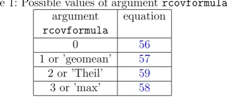
It was explained in section2.3that several different formulas have been proposed to calculate the residual covariance matrix. The user can specify, which formula systemfit should use. Possible values of the argument rcovformula are presented in table 1. By default, systemfit uses equation (57).

Table 1: Possible values of argument rcovformula

argument equation

rcovformula

0 56

1 or ’geomean’ 57

2 or ’Theil’ 59

3 or ’max’ 58

Furthermore, the user can specify whether the means should be subtracted from the resid-uals before (56), (57), (58), or (59) are applied to calculate the residual covariance matrix (see section 2.3). The corresponding argument is called centerResiduals. It must be either “TRUE” (subtract the means) or “FALSE” (take the unmodified residuals). The default value of

4.2.7 3SLS formula

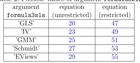
As discussed in sections 2.1 and 2.2, there exist several different formulas to perform a 3SLS estimation. The user can specify the applied formula by the argumentformula3sls. Possible values are presented in table2. The default value is ’GLS’.

Table 2: Possible values of argument formula3sls

argument equation equation

formula3sls (unrestricted) (restricted)

’GLS’ 20 47

’IV’ 23 49

’GMM’ 25 51

’Schmidt’ 27 53

’EViews’ 29 55

4.2.8 Degrees of freedom for t-tests

There exist two different approaches to determine the degrees of freedom to perform t-tests on the estimated parameters (section 2.4). This can be specified with argument probdfsys. If it is TRUE, the degrees of freedom of the whole system are taken. In contrast, if probdfsys is

FALSE, the degrees of freedom of the single equation are taken. By default,probdfsysisTRUE, if any restrictions are specified using either the argumentR.restr or the argumentTX, and it isFALSE otherwise.

4.2.9 Sigma squared

In case of OLS or 2SLS estimations, argumentsingle.eq.sigmacan be used to specify, whether differentσ2

s for each single equation or the sameσ2

for all equations should be used. If argu-ment single.eq.sigmais TRUE, equations (9) and (17) are applied. In contrast, if argument

single.eq.sigmaisFALSE, equations (8) and (16) are applied. By default,single.eq.sigma

is FALSE, if any restrictions are specified using either the argumentR.restr or the argument

TX, and it is TRUEotherwise.

4.2.10 System options

Finally, two options regarding some internal calculations are available. First, argument sol-vetolspecifies the tolerance level for detecting linear dependencies when inverting a matrix or calculating a determinant (using functionssolveand det). The default value depends on the used computer system and is equal to the default tolerance level of solve and det. Second, argument saveMemory can be used in case of large data sets to accelerate the estimation by omitting some calculation that are not crucial for the basic estimation. Currently, only the calculation of McElroy’sR2

is omitted. The default value of argument saveMemoryisTRUE, if the argumentdata is specified and the number of observations times the number of equations is larger than 1000, and it isFALSEotherwise.

4.3 The wrapper function

systemfitClassic

The wrapper functionsystemfitClassic can be applied to (classical) panel-like data in long format6

if the regressors are the same for all equations. This function is called by

> systemfitClassic(method, formula, eqnVar, timeVar, data)

6

The mandatory arguments are method, formula,eqnVar, and timeVar. Argument method

is the same as in systemfit (see section 4.1). The second argument formula is a standard formula inR_{that will be applied to all equations. ArgumenteqnVarspecifies the variable name}

indicating the equation to which the observation belongs, and argumenttimeVarspecifies the variable name indicating the time. Finally, data is a data.frame that contains all required data.

We demonstrate the usage of systemfitClassic using an example taken fromTheil(1971, pp. 295, 300) that is based on Grunfeld (1958). We want to estimate a model for gross investment of 2 US firms in the years 1935–1954:

investit =β1+β2∗value_it+β3∗capital_it (71)

whereinvest is the gross investment of firm iin year t,valueis the market value of the firm at the end of the previous year, andcapitalis the capital stock of the firm at the end of the previous year.

This model can be estimated by

> data("GrunfeldTheil")

> theilSur <- systemfitClassic("SUR", invest ~ value + capital, + "firm", "year", data = GrunfeldTheil)

The first line loads example data that are included with the package. And then, a seemingly unrelated regression is performed, where the variable “firm” indicates the firm and the variable “year” indicates the time.

The function systemfitClassic has also an optional argument pooled that is a logical variable indicating whether the coefficients should be restricted to be equal in all equations. By default, this argument is set to “FALSE”. In addition all optional arguments of systemfit

(see section4.2) except foreqnLabels and TXcan be used with systemfitClassic, too.

4.4 Testing linear restrictions

As described in section2.6, linear restrictions can be tested by an F test, Wald test or LR test. The corresponding functions in packagesystemfitareftest.systemfit,waldtest.systemfit, and lrtest.systemfit, respectively.

We will now test the restriction β2 = −β6 that was specified by the matrix Rmat and the vectorqvec in the example above (p.16).

> ftest.systemfit(fitsur, Rmat, qvec)

F-test for linear parameter restrictions in equation systems F-statistic: 0.9322

degrees of freedom of the numerator: 1 degrees of freedom of the denominator: 33 p-value: 0.3413

> waldtest.systemfit(fitsur, Rmat, qvec)

Wald-test for linear parameter restrictions in equation systems Wald-statistic: 0.6092

degrees of freedom: 1 p-value: 0.4351

> lrtest.systemfit(fitsurRmat, fitsur)

Likelihood-Ratio-test for parameter restrictions in equation systems LR-statistic: 1.004

The linear restrictions are tested by an F test first, then by a Wald test, and finally by an LR test. The functions ftest.systemfit and waldtest.systemfit have three arguments. The first argument must be an unrestricted regression returned by systemfit. The second and third argument are the restriction matrix R and the vector q as described in section 2.2. In contrast, the functionlrtest.systemfitneeds two arguments. The first argument must be a restricted and the second an unrestricted regression returned bysystemfit.

All tests print a short explanation first. Then the empirical test statistic and the degree(s) of freedom are reported. Finally the p-value is printed. While there is some variation of the p-values across the three different tests, all tests suggest the same decision: The null hypothesis

β2 =−β6 cannot be rejected at any reasonable level of significance.

4.5 Hausman test

A Hausman test, which is described in section2.7, can be carried out with following commands: > fit2sls <- systemfit("2SLS", list(demand = eqDemand, supply = eqSupply), + inst = ~income + farmPrice + trend, data = Kmenta)

> fit3sls <- systemfit("3SLS", list(demand = eqDemand, supply = eqSupply), + inst = ~income + farmPrice + trend, data = Kmenta)

> hausman.systemfit(fit2sls, fit3sls)

Hausman specification test for consistency of the 3SLS estimation

data: Kmenta

Hausman = 2.5357, df = 7, p-value = 0.9244

First of all, the model is estimated by 2SLS and then by 3SLS. Finally, in the last line the test is carried out by the command hausman.systemfit. This function requires two arguments: the result of a 2SLS estimation and the result of a 3SLS estimation. The Hausman test statistic is 2.536, which has aχ2

distribution with 7 degrees of freedom under the null hypothesis. The corresponding p-value is 0.924. This shows that the null hypothesis is not rejected at any reasonable level of significance. Hence, we can assume that the 3SLS estimator is consistent.

5 Testing reliability

In this section we test the reliability of the results fromsystemfitand systemfitClassic.

5.1 Kmenta (1986): Example on p. 685 (food market)

First, we reproduce an example taken from Kmenta (1986, p. 685). The data are available from Table 13-1 (p. 687), and the results are presented in Table 13-2 (p. 712) of this book.

Before starting the estimation, we load the data and specify the two formulas to estimate as well as the instrumental variables. Then the equation system ist estimated by OLS, 2SLS, 3SLS, and iterated 3SLS. After each estimation the estimated coefficients are reported.

> data("Kmenta")

> eqDemand <- consump ~ price + income

> eqSupply <- consump ~ price + farmPrice + trend > inst <- ~income + farmPrice + trend

> system <- list(demand = eqDemand, supply = eqSupply)

OLS estimation:

Estimate Std. Error t value Pr(>|t|) eq 1 (Intercept) 99.8954 7.5194 13.2851 0.0000 eq 1 price -0.3163 0.0907 -3.4882 0.0028 eq 1 income 0.3346 0.0454 7.3673 0.0000 eq 2 (Intercept) 58.2754 11.4629 5.0838 0.0001 eq 2 price 0.1604 0.0949 1.6901 0.1104 eq 2 farmPrice 0.2481 0.0462 5.3723 0.0001 eq 2 trend 0.2483 0.0975 2.5462 0.0216

2SLS estimation:

> fit2sls <- systemfit("2SLS", system, inst = inst, data = Kmenta) > round(coef(summary(fit2sls)), digits = 4)

Estimate Std. Error t value Pr(>|t|) eq 1 (Intercept) 94.6333 7.9208 11.9474 0.0000 eq 1 price -0.2436 0.0965 -2.5243 0.0218 eq 1 income 0.3140 0.0469 6.6887 0.0000 eq 2 (Intercept) 49.5324 12.0105 4.1241 0.0008 eq 2 price 0.2401 0.0999 2.4023 0.0288 eq 2 farmPrice 0.2556 0.0473 5.4096 0.0001 eq 2 trend 0.2529 0.0997 2.5380 0.0219

3SLS estimation:

> fit3sls <- systemfit("3SLS", system, inst = inst, data = Kmenta) > round(coef(summary(fit3sls)), digits = 4)

Estimate Std. Error t value Pr(>|t|) eq 1 (Intercept) 94.6333 7.9208 11.9474 0.0000 eq 1 price -0.2436 0.0965 -2.5243 0.0218 eq 1 income 0.3140 0.0469 6.6887 0.0000 eq 2 (Intercept) 52.1972 11.8934 4.3888 0.0005 eq 2 price 0.2286 0.0997 2.2934 0.0357 eq 2 farmPrice 0.2282 0.0440 5.1861 0.0001 eq 2 trend 0.3611 0.0729 4.9546 0.0001

Iterated 3SLS estimation:

> fitI3sls <- systemfit("3SLS", system, inst = inst, data = Kmenta,

+ maxit = 250)

> round(coef(summary(fitI3sls)), digits = 4)

Estimate Std. Error t value Pr(>|t|) eq 1 (Intercept) 94.6333 7.9208 11.9474 0.0000 eq 1 price -0.2436 0.0965 -2.5243 0.0218 eq 1 income 0.3140 0.0469 6.6887 0.0000 eq 2 (Intercept) 52.6618 12.8051 4.1126 0.0008 eq 2 price 0.2266 0.1075 2.1086 0.0511 eq 2 farmPrice 0.2234 0.0468 4.7756 0.0002 eq 2 trend 0.3800 0.0720 5.2771 0.0001

5.2 Greene (2003): Example 15.1 (Klein’s model I)

Second, we try to replicate Klein’s Model I (Klein, 1950) that is described in Greene (2003, pp. 381). The data are available from the online complements to Greene (2003), Table F15.1 (http://pages.stern.nyu.edu/~wgreene/Text/econometricanalysis.htm), and the esti-mation results are presented in Table 15.3 (p. 412).

Initially, the data are loaded and three equations as well as the instrumental variables are specified. As in the example before, the equation system ist estimated by OLS, 2SLS, 3SLS, and iterated 3SLS, and estimated coefficients of each estimation are reported.

> data("KleinI")

> eqConsump <- consump ~ corpProf + corpProfLag + wages > eqInvest <- invest ~ corpProf + corpProfLag + capitalLag > eqPrivWage <- privWage ~ gnp + gnpLag + trend

> inst <- ~govExp + taxes + govWage + trend + capitalLag + corpProfLag +

+ gnpLag

> system <- list(Consumption = eqConsump, Investment = eqInvest, + "Private Wages" = eqPrivWage)

OLS estimation:

> kleinOls <- systemfit("OLS", system, data = KleinI) > round(coef(summary(kleinOls)), digits = 3)

Estimate Std. Error t value Pr(>|t|) eq 1 (Intercept) 16.237 1.303 12.464 0.000 eq 1 corpProf 0.193 0.091 2.115 0.049 eq 1 corpProfLag 0.090 0.091 0.992 0.335 eq 1 wages 0.796 0.040 19.933 0.000 eq 2 (Intercept) 10.126 5.466 1.853 0.081 eq 2 corpProf 0.480 0.097 4.939 0.000 eq 2 corpProfLag 0.333 0.101 3.302 0.004 eq 2 capitalLag -0.112 0.027 -4.183 0.001 eq 3 (Intercept) 1.497 1.270 1.179 0.255 eq 3 gnp 0.439 0.032 13.561 0.000 eq 3 gnpLag 0.146 0.037 3.904 0.001 eq 3 trend 0.130 0.032 4.082 0.001

2SLS estimation:

> klein2sls <- systemfit("2SLS", system, inst = inst, data = KleinI,

+ rcovformula = 0)

> round(coef(summary(klein2sls)), digits = 3)

3SLS estimation:

> klein3sls <- systemfit("3SLS", system, inst = inst, data = KleinI,

+ rcovformula = 0)

> round(coef(summary(klein3sls)), digits = 3)

Estimate Std. Error t value Pr(>|t|) eq 1 (Intercept) 16.441 1.305 12.603 0.000 eq 1 corpProf 0.125 0.108 1.155 0.264 eq 1 corpProfLag 0.163 0.100 1.624 0.123 eq 1 wages 0.790 0.038 20.826 0.000 eq 2 (Intercept) 28.178 6.794 4.148 0.001 eq 2 corpProf -0.013 0.162 -0.081 0.937 eq 2 corpProfLag 0.756 0.153 4.942 0.000 eq 2 capitalLag -0.195 0.033 -5.990 0.000 eq 3 (Intercept) 1.797 1.116 1.611 0.126 eq 3 gnp 0.400 0.032 12.589 0.000 eq 3 gnpLag 0.181 0.034 5.307 0.000 eq 3 trend 0.150 0.028 5.358 0.000

iterated 3SLS estimation:

> kleinI3sls <- systemfit("3SLS", system, inst = inst, data = KleinI,

+ rcovformula = 0, maxit = 500)

> round(coef(summary(kleinI3sls)), digits = 3)

Estimate Std. Error t value Pr(>|t|) eq 1 (Intercept) 16.559 1.224 13.524 0.000 eq 1 corpProf 0.165 0.096 1.710 0.105 eq 1 corpProfLag 0.177 0.090 1.960 0.067 eq 1 wages 0.766 0.035 22.031 0.000 eq 2 (Intercept) 42.896 10.594 4.049 0.001 eq 2 corpProf -0.357 0.260 -1.370 0.188 eq 2 corpProfLag 1.011 0.249 4.065 0.001 eq 2 capitalLag -0.260 0.051 -5.115 0.000 eq 3 (Intercept) 2.625 1.196 2.195 0.042 eq 3 gnp 0.375 0.031 12.050 0.000 eq 3 gnpLag 0.194 0.032 5.977 0.000 eq 3 trend 0.168 0.029 5.805 0.000

Again, the results show that systemfit returns the same results as published in Greene

(2003).7

Also in this case we have two minor deviations, where only the last digit is different.

5.3 Theil (1971): Example on p. 295 (General Electric and

Westinghouse)

Third, we estimate an example taken fromTheil(1971, p. 295) that is based onGrunfeld(1958). The data are available from Table 7.1 (p. 296), and the results are presented on pages 295 and 300 of this book.

After loading the data and specifying the formula, the model is estimated by OLS and SUR. The coefficients of each estimation are reported.

> data("GrunfeldTheil")

> formulaGrunfeld <- invest ~ value + capital

7

OLS estimation (page 295)

> theilOls <- systemfitClassic("OLS", formulaGrunfeld, "firm", + "year", data = GrunfeldTheil)

> round(coef(summary(theilOls)), digits = 3)

Estimate Std. Error t value Pr(>|t|) eq 1 (Intercept) -9.956 31.374 -0.317 0.755 eq 1 value.General.Electric 0.027 0.016 1.706 0.106 eq 1 capital.General.Electric 0.152 0.026 5.902 0.000 eq 2 (Intercept) -0.509 8.015 -0.064 0.950 eq 2 value.Westinghouse 0.053 0.016 3.368 0.004 eq 2 capital.Westinghouse 0.092 0.056 1.647 0.118

SUR estimation (page 300)

> theilSur <- systemfitClassic("SUR", formulaGrunfeld, "firm", + "year", data = GrunfeldTheil, rcovformula = 0)

> round(coef(summary(theilSur)), digits = 3)

Estimate Std. Error t value Pr(>|t|) eq 1 (Intercept) -27.719 27.033 -1.025 0.320 eq 1 value.General.Electric 0.038 0.013 2.883 0.010 eq 1 capital.General.Electric 0.139 0.023 6.036 0.000 eq 2 (Intercept) -1.252 6.956 -0.180 0.859 eq 2 value.Westinghouse 0.058 0.013 4.297 0.000 eq 2 capital.Westinghouse 0.064 0.049 1.308 0.208

The functionsystemfitClassic, which is a wrapper function tosystemfitreturns exactly the same results as published in Theil(1971, pp. 295, 300).

5.4 Greene (2003): Example 14.1 (Grunfeld’s investment data)

Finally, we reproduce Example 14.1 of Greene (2003, p. 340) that is also based on Grunfeld

(1958). The data are available from the online complements to Greene (2003), Table F13.1 (http://pages.stern.nyu.edu/~wgreene/Text/econometricanalysis.htm), and the esti-mation results are presented in Tables 14.1 and 14.2 (p. 351).

First, we load the data and specify the formula to estimate. Then, the systems is estimated by OLS, pooled OLS, SUR, and pooled SUR. Immediately after each estimation, the estimated coefficients are reported. Furthermore, theσ2

values of the OLS estimations, and the residual covariance matrix as well as the residual correlation matrix of the SUR estimations are printed.

> data("GrunfeldGreene")

> formulaGrunfeld <- invest ~ value + capital

OLS estimation (Table 14.2):

> greeneOls <- systemfitClassic("OLS", formulaGrunfeld, "firm", + "year", data = GrunfeldGreene)

> round(coef(summary(greeneOls)), digits = 4)

eq 3 (Intercept) -149.7825 105.8421 -1.4151 0.1751 eq 3 value.General.Motors 0.1193 0.0258 4.6172 0.0002 eq 3 capital.General.Motors 0.3714 0.0371 10.0193 0.0000 eq 4 (Intercept) -30.3685 157.0477 -0.1934 0.8490 eq 4 value.US.Steel 0.1566 0.0789 1.9848 0.0635 eq 4 capital.US.Steel 0.4239 0.1552 2.7308 0.0142 eq 5 (Intercept) -0.5094 8.0153 -0.0636 0.9501 eq 5 value.Westinghouse 0.0529 0.0157 3.3677 0.0037 eq 5 capital.Westinghouse 0.0924 0.0561 1.6472 0.1179

> round(sapply(greeneOls$eq, function(x) {

+ return(x$ssr/20)

+ }), digits = 3)

[1] 149.872 660.829 7160.294 8896.416 88.662

pooled OLS (Table 14.2):

> greeneOlsPooled <- systemfitClassic("OLS", formulaGrunfeld, "firm", + "year", data = GrunfeldGreene, pooled = TRUE)

> round(coef(summary(greeneOlsPooled$eq[[1]])), digits = 4)

Estimate Std. Error t value Pr(>|t|) (Intercept) -48.0297 21.4802 -2.2360 0.0276 value.Chrysler 0.1051 0.0114 9.2360 0.0000 capital.Chrysler 0.3054 0.0435 7.0186 0.0000

> sum(sapply(greeneOlsPooled$eq, function(x) {

+ return(x$ssr)

+ }))/100

[1] 15708.84

SUR estimation (Table 14.1):

> greeneSur <- systemfitClassic("SUR", formulaGrunfeld, "firm", + "year", data = GrunfeldGreene, rcovformula = 0)

> round(coef(summary(greeneSur)), digits = 4)

Estimate Std. Error t value Pr(>|t|) eq 1 (Intercept) 0.5043 11.5128 0.0438 0.9656 eq 1 value.Chrysler 0.0695 0.0169 4.1157 0.0007 eq 1 capital.Chrysler 0.3085 0.0259 11.9297 0.0000 eq 2 (Intercept) -22.4389 25.5186 -0.8793 0.3915 eq 2 value.General.Electric 0.0373 0.0123 3.0409 0.0074 eq 2 capital.General.Electric 0.1308 0.0220 5.9313 0.0000 eq 3 (Intercept) -162.3641 89.4592 -1.8150 0.0872 eq 3 value.General.Motors 0.1205 0.0216 5.5709 0.0000 eq 3 capital.General.Motors 0.3827 0.0328 11.6805 0.0000 eq 4 (Intercept) 85.4233 111.8774 0.7635 0.4556 eq 4 value.US.Steel 0.1015 0.0548 1.8523 0.0814 eq 4 capital.US.Steel 0.4000 0.1278 3.1300 0.0061 eq 5 (Intercept) 1.0889 6.2588 0.1740 0.8639 eq 5 value.Westinghouse 0.0570 0.0114 5.0174 0.0001 eq 5 capital.Westinghouse 0.0415 0.0412 1.0074 0.3279

Chrysler General Electric General Motors US Steel Chrysler 152.849 2.047 -313.704 455.089 General Electric 2.047 700.456 605.336 1224.405 General Motors -313.704 605.336 7216.044 -2686.517 US Steel 455.089 1224.405 -2686.517 9188.151 Westinghouse 16.661 200.316 129.887 652.716

Westinghouse

Chrysler 16.661

General Electric 200.316 General Motors 129.887

US Steel 652.716

Westinghouse 94.912

> round(summary(greeneSur)$rcor, digits = 3)

Chrysler General Electric General Motors US Steel Westinghouse

Chrysler 1.000 0.006 -0.299 0.384 0.138

General Electric 0.006 1.000 0.269 0.483 0.777 General Motors -0.299 0.269 1.000 -0.330 0.157

US Steel 0.384 0.483 -0.330 1.000 0.699

Westinghouse 0.138 0.777 0.157 0.699 1.000

pooled SUR estimation (Table 14.1):

> greeneSurPooled <- systemfitClassic("WSUR", formulaGrunfeld,

+ "firm", "year", data = GrunfeldGreene, pooled = TRUE, rcovformula = 0) > round(coef(summary(greeneSurPooled$eq[[1]])), digits = 4)

Estimate Std. Error t value Pr(>|t|) (Intercept) -28.2467 4.8882 -5.7785 0 value.Chrysler 0.0891 0.0051 17.5663 0 capital.Chrysler 0.3340 0.0167 19.9859 0

> round(greeneSurPooled$rcov, digits = 3)

Chrysler General Electric General Motors US Steel Chrysler 305.610 -1966.648 -4.805 2158.595 General Electric -1966.648 34556.603 -7160.667 -28722.006 General Motors -4.805 -7160.667 10050.525 4439.989 US Steel 2158.595 -28722.006 4439.989 34468.976 Westinghouse -123.920 4274.000 -1400.747 -2893.733

Westinghouse Chrysler -123.920 General Electric 4274.000 General Motors -1400.747 US Steel -2893.733 Westinghouse 833.357

> round(cov(residuals(greeneSurPooled)), digits = 3)

Chrysler General Electric General Motors US Steel Chrysler 167.403 174.038 -432.370 260.431 General Electric 174.038 3733.260 -1322.236 -972.145 General Motors -432.370 -1322.236 9396.058 -897.950 US Steel 260.431 -972.145 -897.950 10052.045 Westinghouse 89.336 1302.231 -865.791 -180.385

Chrysler 89.336 General Electric 1302.231 General Motors -865.791 US Steel -180.385 Westinghouse 564.156

> round(summary(greeneSurPooled)$rcor, digits = 3)

Chrysler General Electric General Motors US Steel Westinghouse

Chrysler 1.000 0.220 -0.345 0.201 0.291

General Electric 0.220 1.000 -0.223 -0.159 0.897 General Motors -0.345 -0.223 1.000 -0.092 -0.376

US Steel 0.201 -0.159 -0.092 1.000 -0.076

Westinghouse 0.291 0.897 -0.376 -0.076 1.000

For this example, the function systemfitClassic returns nearly the same results as pub-lished inGreene(2003).8

Two different residual covariance matrices of the pooled SUR estima-tion are presented. The first is calculated without centering the results (see secestima-tion 2.3). It is equal to the one published in the book (Greene,2003, p. 351). The second residual covariance matrix is calculated after centering the results. It is equal to the one published in the errata (http://pages.stern.nyu.edu/~wgreene/Text/econometricanalysis.htm).

6 Summary and outlook

In this article, we have described some of the basic features of the systemfitpackage for esti-mation of linear systems of equations. Many details of the estiesti-mation can be controlled by the user. Furthermore, the package provides some statistical tests for parameter restrictions and consistency of 3SLS estimation. It has been tested on a variety of datasets and has produced satisfactory for a few years. While the systemfit package performs the basic fitting methods, more sophisticated tools exist. We hope to implement missing functionalities in the near future.

Unbalanced datasets

Currently, thesystemfitpackage requires that all equations have the same number of observa-tions. However, many data sets have unbalanced observaobserva-tions.9

Simply dropping data points that do not contain observations for all equations may reduce the number of observations con-siderably, and thus, the information utilized in the estimation. Hence, it is our intention to include the capability for estimations with unbalanced data sets as described inSchmidt(1977) in future releases ofsystemfit.

Serial correlation and heteroscedasticity

For all of the methods developed in the package, the disturbances of the individual equations are assumed to be independent and identically distributed (iid). The package could be en-hanced by the inclusion of methods to fit equations with serially correlated and heteroscedastic disturbances (Parks,1967).

8

There are several typos and errors in Table 14.1 (p. 412). Please take a look at the errata of this book (http: //pages.stern.nyu.edu/~wgreene/Text/econometricanalysis.htm).

9

Estimation methods

In the future, we wish to include more sophisticated estimation methods such as limited-information maximum likelihood (LIML), full-limited-information maximum likelihood (FIML), gen-eralized methods of moments (GMM) and spatial econometric methods.

Non-linear estimation

Finally, thesystemfitpackage provides a function to estimate systems of non-linear estimations. However, the functionnlsystemfitis currently under development and the results are not yet always reliable due to convergence difficulties.

References

Bates D (2004). “Least Squares Calculations in R.”R News,4(1), 17–20. URLhttp://CRAN. R-project.org/doc/Rnews/.

Greene WH (2003). Econometric Analysis. Prentice Hall, 5th edition.

Greene WH (2006). “Information about SUR estimation in LIMDEP.” Personal email on 2006/02/16.

Grunfeld Y (1958). The Determinants of Corporate Investment. Ph.D. thesis, University of Chicago.

Hausman JA (1978). “Specification Test in Econometrics.”Econometrica,46, 1251–1272.

Judge GG, Griffiths WE, Hill RC, L¨utkepohl H, Lee TC (1985). The Theory and Practice of Econometrics. John Wiley and Sons, 2nd edition.

Klein L (1950). Economic Fluctuations in the United States, 1921–1941. John Wiley, New York.

Kmenta J (1986). Elements of econometrics. Macmillan, New York, 2 edition.

McElroy MB (1977). “Goodness of Fit for Seemingly Unrelated Regressions.” Journal of Econometrics,6, 381–387.

Parks RW (1967). “Effcient estimation of a system of regression equations when disturbances are both serially and contemporaneously correlated.” Journal of the American Statistical Association,62, 500–509.

R Development Core Team (2005). R: A language and environment for statistical computing. R Foundation for Statistical Computing, Vienna, Austria. ISBN 3-900051-07-0, URLhttp: //www.R-project.org.

Schmidt P (1977). “Estimation of Seemingly Unrelated Regressions with Unequal Numbers of Observations.” Journal of Econometrics,5, 365–377.

Schmidt P (1990). “Three-Stage Least Squares with Different Instruments for Different Equa-tions.” Journal of Econometrics,43, 389–394.

Theil H (1971). Principles of Econometrics. Wiley, New York.

Zellner A, Huang DS (1962). “Further Properties of Efficient Estimators for Seemingly Unre-lated Regression Equations.” International Economic Review,3(3), 300–313.