Difference based Non Linear Fractals using IFS

Difference based Non-Linear Fractals using IFS

B Dinesh Rao

Associate Professor SOIS, Manipal Manipal University

Deepak Rao B

Assistant Professor (Sel grade) SOIS, Manipal

Manipal University

U C Niranjan,

Ph.D

Training, MDN Manipal

ABSTRACT

Fractals are self-similar images. There are many techniques for generating fractals. IFS are one of them. IFS use a set of linear transformations for generation of fractals. We propose a method of modifying IFS such that non-linear transformations can be used for generating pleasant looking fractals. We also show a technique which ensures convergence of the fractal Images.

Non-linear fractals have been developed by Frederic Raynal, Evelyne, Lutton and Pierre Collet [1]. It is difficult to ensure that convergence using their method. Our method is similar to the one in IFS and very easily understandable [2]. Fractal compression is also one of the important compression techniques [3].

Keywords

IFS, Fractals, non-linear

1.

INTRODUCTION

The use of a system of affine transforms to define a fractal object has been described by Barnsley [4]. A system of transforms Wi can be written as [4]

Wi: Z  Ti Z + Vi

Where

T = a b V = e

c d f

and

Z = x

y

That is if Z = x

y

then x = ax + by +e

y = cx + dy + f

The set of transforms need to be contractive and there exists a unique attractor set containing infinitely many points Z. For graphical purposes we say that there is a fixed set of pixels which approximate this attractor [5][6].

Our proposed technique is intended to extend the transforms to be non-linear. We wish to demonstrate that a set of non– linear transforms also generate a unique attractor set comprising of infinite points.

A set of transforms can be made non-linear by converting the transforms to the form

x  a xn _{+ b x}n-1 _{+ …. + k x}0

or

x  a Sin(x) + b Cos(x) + ….

or

x  a Kx

+ b Ly + ….

It will be demonstrated that the usage of the above equations also generate fractals.

2.

MATERIAL AND METHODS

We will first look at a method for generating IFS. Consider the following three transformations

1. x= 0.5 x + 0

y = 0.5y + 0

2. x =0.5x + 0

y = 0.5y + 150

3. x = 0.5x + 150

y= 0.5y +0 (Equation 1)

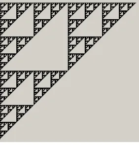
Select an arbitrary point x, y and select one of the three affine transformations in random, apply it to the point x, y we get a new point x’, y’. If the above procedure is repeated on the point x’, y’, we get a new point x”, y”.

39

Figure 1: Sierpensky’s triangle

The C code for simple IFS is given below.

for(i=0;i<95000;i++) {

ran=rand()%3;

switch(ran) {

case 0:

x = 0.5 * x + 0;

y = 0.5 * y + 0;

break;

case 1:

x = 0.5 * x + 0;

y = 0.5 * y + 150;

break;

case 2:

x = 0.5 * x + 150;

y = 0.5 * y + 0;

break;

}

putpixel(x,y,1)

}

The result is the following fractal. It is called the Sierpensky’s triangle.

The affine transformations are of the form

x’ = ax + by + c

and y’ = dx + ey + f

Six numbers are used to represent a transformation {a,b,c,d,e,f}[2]. Hence, the above example would have {0.5,0,0,0,0.5,0},{0.5,0,0,0,0.5,150}, (0.5,0,150,0,0.5,0} representing the three transforms.

2.1

IFS Variant

IFS methodology is modified slightly to get meaningful images in a more intuitive way. We will call this method IFS-variant.

We obtain an invariable point for every transformation i.e., x’ = x and y’ = y.

Let us consider the above three transformations (Equation 1). We notice that the invariant points are (300,300), (0,300)and (300,300)for the three transforms respectively.

Given an invariant point, we develop IFS like equations are developed as follows

x= x+ (invariant(x) –x)*a + b

y = y +(invariant(y) – y)*c + d

Compute the new point as a linear function of distance between the current point and the invariant point.

Our equations will be

1. x = x + (300 – x) * 0.5 + 0

y = y + (300 - x) * 0.5 + 0

2. x = x + (0 – x) * 0.5 + 0

y = y + (300 – x) * 0.5 + 0

3. x = x + (300 – x) * 0.5 + 0

y = y + (0 – x) * 0.5 + 0

The method similar to IFS is used to generate the set of points. Select an arbitrary point x, y and select one of the three affine transformations in random, apply it to the point x, y and get a new point x’, y’. If the above procedure is repeated on the point x’, y’, we get a new point x”, y” and so on for some number of iterations, say 100000. Figure 1 is a result of the equations shown above.

2.2

Non linear IFS

We attempt to generate a non linear IFS with quadratic values. We change the equation to involve x2 _{and y}2 _{terms. x and y}

values are normalized by dividing with 500 so that the square terms do not diverge.

C code for IFS Non-Linear

case 0:

x = 175*x/500*x/500 + 75*x/500+100;

y = 175*y/500 * y/500 + 75*y/500+220;

break;

case 1:

y = 175*y/500 * y/500 + 75*y/500+50;

break;

case 2:

x = 175*x/500*x/500 + 75*x/500+50;

y = 175*y/500 * y/500 + 75*y/500+50;

break;

.

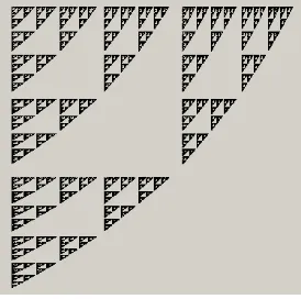
Figure 2: IFS non-linear

In Figure 2 we have generated IFS non-linear with the program above. We find it difficult to interpret and generate the image intuitively. Hence we use IFS variant further in this paper to develop non - linear IFS.

2.3

Non-linear Variant

If we extend the equations to higher order transformations, ensuring contractivity would be a problem. We can divide x and y by suitable values so that they are within the range 0 to 1 and ensure convergence. Hence we divide x and y by largest possible values that they can take. We will now try to generate variants of the Sierpensky’s triangle (Figure 1) to obtain a few non linear fractals. The largest x-distance from any invariant point is 300 and the largest y-distance from any invariant point is 300. If we divide x and y by a value greater than 300 and scale them back appropriately, we get good non linear fractals.

Here are a few equations and their corresponding images. In the following discussion we consider the following invariant points implying that we have three transforms.

1. 0,0

2. 300,0

3. 0,300

We use the following values of ‘p’ and ‘q’ in our examples.

p = invariant(x) - x

q = invariant(y) - y

We note that all the three transformations are identical in all the cases. The only difference will be in p and q values.

1) Quadratic:

These equations are of the form

x = ax2 + bx + c

y = dy2 + ey +f

Consider the following transformations

x = x + p*0.5 + p/500 * p/500 * 60

y = y + q*0.5 + q/500 * q/500 * 60

Figure 3 : Quadratic non-linear IFS

2) Cubic:

These equations are of the form

x = ax3 + bx2 + cx + d

y = ey3 _{+ fy}2 _{+ gy + h}

Consider the following transformations

x = x + p*0.5+ p/500 *p/500 *p/500 *60

y = y + q*0.5 + q/500 *q/500 *q/500*60

Fig 4: Cubic non-linear IFS

41 These equations are of the form

x = abx + cx + d

y = efy + gy + h

Consider the following transformations

x = x + p*0.5 + pp _{* 30}

y = y + q*0.5 +qp _{* 30}

Figure 5: Exponential non-linear IFS

4) Convergence:

When ensuring convergence for linear fractals in ifs-variants, we have to have the scaling factor between 0 and 1. that is, if p is the distance from the fixed point, constant * p should be such that the new point will not go outside the convex hull of the invariant points.

If x = a p + b is the equation, the new value of ‘a’ should be between 0 and 1.

Now, while extending these thoughts to non-linear equation, if x = a p + b p2 + c is the expected equation, we divide one p by the largest distance from the variant point in the quadratic term. Hence we write x = a p + b p * p/350 +c. If a+b is less than 1, it converges.

Let us now extend this to cubic equation,

x = ap+b p*p/350+c p*p/350* p/350+d.

now, a+b+c should be less than 1.

Hence we have established a simple criteria for convergence of non-linear fractals.

3.

APPLICATIONS

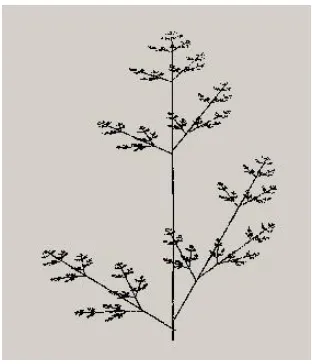
Linear and non-linear fractals can be used to generate a wide range of good-looking figures which can be used on fabrics. Non-linear fractals can also be used to compress images. The three images below demonstrate as to how non-linearity can be induced into existing linear fractals. Figure 6 is a linear fractal designed using four invraiant points or transforms. A non-linear component of square term has been added to the second transform to generate figure 7. It can be seen that the left branch has curved in figure 7 which is not seen in figure

6. Non-linearity has been introduced as a cubic quantity in figure 8. The nature of curvature is different in these two images. The curvature is reflected in all the branches demonstrating the fractal nature of the images. More curvature can be introduced if a larger non-linear component is added.

Figure 6: linear twig

Figure 7:Non-linear twig (quadratic)

4.

RESULTS AND DISCUSSION

The variant of IFS (IFS-variant) seems to be more powerful than IFS since we are dealing with individual distances in the transformations while in IFS we use the same x and y values for all transformations. However we have been able to identify IFS for most of the images developed using the IFS-variant. Another advantage of the variant is the ease of expecting and understanding the images. Let us consider the nonlinear quadratic transformations (Figure 3). As we go away from the invariant point, we see greater curvature and that is the curve expected from a quadratic equation.

To generate IFS we need not restrict the transformations to be affine. Any appropriate set of non-linear transforms would also generate fractals. We see that we can apply a wide range of polynomial, exponentials which generate pleasing fractals. Use of nonlinear transforms also gives us an insight into the graphical nature of these transformations. Till now we have only seen the visual effects of linear transformations. We only have to note that we can extend non linear transformations to higher dimensional fractals and expect similar results.

5.

REFERENCES

[1] Frederic Raynal, Evelyne, Lutton, Pierre Collet, Manipulation of Non-Linear IFS Attractors Using Genetic Programming (1999), Proceedings of the Congress on Evolutionary Computation.

[2] Dinesh Rao B, Deepak Rao, Niranjan U.C, Non-linear Fractals using IFS, NCIS, NCKBFT-07, Manipal University, 2007.

[3] Barnsley, A better way to compress images, Byte, January 1988.

[4] Barnsley, Fractals everywhere, Academic Press 1988.

[5] Lu Ning, Fractal Imaging, academic Press 1997.