Globalization and Environment: Can Pollution Haven Hypothesis alone explain the impact of Globalization on Environment?

Munich Personal RePEc Archive

Globalization and Environment: Can

Pollution Haven Hypothesis alone

explain the impact of Globalization on

Environment?

Dinda, Soumyananda

S. R. Fatepuria College, Beldanga, Murshidabad, WB, India, ERU,

Indian Statistical Institute, Kolkata, India

15 August 2006

Globalization and Environment: Can Pollution Haven Hypothesis alone explain the impact of Globalization on Environment?

Soumyananda Dinda*

S. R. Fatepuria College, Beldanga, Murshidabad, WB, India. Economic Research Unit, Indian Statistical Institute, Kolkata, India.

First Preliminary Draft: October 15, 2006

Abstract

The economic literature on trade and environment seeks empirically test hypotheses

about how trade affects the environment that is crucial for resolving current policy

debates. Applying panel data technique we examine the impacts of globalization on

pollution level, pollution intensity and relative change of pollution for the developed

(OECD) and developing (Non-OECD) country groups and the world as a whole. This

paper examines the factor endowment and pollution haven hypotheses that predict how

trade affects the environment. Interaction effects also play a crucial role to determine the

impact of globalization on environment. In this study we use CO2 emission and observe

that the impact of globalization on environment heavily depends on the basic

characteristics of a country and its dominating comparative advantage. The empirical

results suggest that globalization increases CO2 emission, which is the main culprit of the

global warming.

JELClassification Number: Q00, F1

Key Words: Globalization, pollution haven hypothesis, factor endowment hypothesis, and interaction effect.

---*C/o, Dipankor Coondoo, Economic Research Unit, Indian Statistical Institute, 203, B. T. Road, Kolkata –

1. Introduction

Economic development through rapid industrialization and growing

environmental consciousness together have generated a heated debate on how economic

development (or growth) is linked with environment. The linkage of environmental

quality with economic development evoked much discussion in the last decade (i.e.,

1990s). The World Development Report (World Bank 1992) presented cross-sectional

evidences on the relationship between different indicators of environmental quality and

per capita national income across countries. Other studies (e.g. Grossman and Krueger,

1991; Selden and Song, 1994; Rothman, 1998; Suri and Chapman, 1998; etc)

documented an inverted U-shaped relationship between environmental degradation and

income. The common point of all these studies is the assertion that environmental

degradation increases initially, reaches a maximum level and after that declines as an

economy develops. This systematic inverted-U relationship has been termed as the

Environmental Kuznets Curve (EKC) following the work of Kuznets (1955), who

postulated a similar relationship between income inequality and economic development.

The EKC relates to the issue of the impacts of economic growth or development on the

environment of a country.

Now automatically one important question arises whether cross border integration

(i.e., globalization) helps or hurts this process. This is indeed the primary motivation for

this study. The aim of this paper is to explore whether globalization hurts the

environment. Applying panel data technique we examine the impacts of globalization on

pollution level, pollution intensity and relative change of pollution for the developed

study we use CO2 emission and observe that the impact of globalization on environment

heavily depends on the characteristics of the economy. The basic characteristics of a

country and its dominating comparative advantage determine how trade liberalization

influences its sectoral composition and consequently environmental outcomes.

This analysis has been done mostly by applying the technique of panel data

analysis to a cross-country panel data set on per capita income and CO2 emission. In what

follows, we explain first the background of this study, methodological framework and

then present the empirical results of our analysis. The paper is organized as follows:

Section 2 presents the background of this study and ideas develop how the globalization

links up environmental quality. Section 3 describes the data set. The empirical results are

presented in Section 4. Finally, in Section 5 some concluding observations have been

drawn.

2. Background of this study

Environmental quality could decline through the scale effect as increasing trade

volume (especially export) would expand the size of the economy thereby increasing the

extent of pollution. Thus, trade might be a cause of environmental degradation, ceteris

paribus. Many economists have long argued that trade is not the root cause of

environmental damage (Birdsall and Wheeler 1993, Lee and Roland-Host 1997, Jones et

al. 1995). However, free trade has the contradictory impacts on environment, both

increasing pollution and motivating reductions in it. Antweiler et al. (2001) and Liddle

(2001) argue that trade may be good for environment. Trade may improve the

environmental quality through technological effect. As income rises through trade,

trade relates one country with international communities, one underdeveloped economy

may rely on technology transfer through foreign direct investment that may reduce

pollution.

However, globalization, by increasing competition for investment, may trigger the

environmental race to bottom (Wheeler (2000)). Poor economies may be able to improve

their environmental quality as investment raise their income levels. Thus, globalization

may facilitate pollution reduction. In fact, the bottom rises with economic growth. Tisdell

(2001) points out that globalization can be a driving force for global economic growth.

Yet opinion is divided about the benefits of this process. The global economy raises the

issue of potential conflicts between two powerful current trends – viz., the worldwide

acceptance of market oriented economic reform process on the one hand, and

environmental protection on the other.

It should be mentioned that a polluting activity in a high-income country normally

faces higher regulatory costs1 than its counterpart in a developing country (Mani and

Wheeler (1998)). Under these circumstances the pollution intensive industries will have a

natural tendency to migrate to countries with weaker environmental regulations

(Copeland and Taylor (1995)). This is referred to as the Pollution Haven Hypothesis

(PHH) (See, Bommer (1999), Cole (2003, 2004)). The PHH refers to the possibility that

polluting industries concentrate in developing countries with low environmental

standards. The pollution haven hypothesis (PHH) predicts that, under free trade,

multinational firms will relocate the production of their polluting goods to developing

1

countries, taking advantage of the low environment monitoring in these countries.

Developing countries will develop a comparative advantage in pollution-intensive

industries and become ‘haven’ for the world’s polluting industries. Thus, developed

countries are expected to benefit in terms of environmental quality from trade, while

developing countries will lose (See Figure 1). In other words, the PHH basically

suggests that countries having stricter environmental standard will lose all the dirty

industries and poor countries (i.e., those having poorer environmental standard) will get

them all. It is also true that the differences in the consumer preferences for a cleaner

environment in rich and poor countries also induce the displacement hypothesis and/or

PHH.

It is observed that changes in the structure of production in developed economies

are not accompanied by equivalent changes in the structure of consumption. This could

be explained by the EKC, which actually record the shifting of dirty industries to less

developed economies. As Rothman (1998) speculates, what appears to be an

improvement in environmental quality may in reality be an indicator of increased ability

of consumers in wealthy nations to distance themselves from the environmental

degradation associated with their consumption. The mechanisms through which such

distancing take place may include both moving sources of pollution away from the

people and moving people away from pollution sources2. Thus, in general, the

phenomenon of distancing may be a possible source of EKC results. Hettige et al (1992)

observe that toxic intensity grew rapidly in high-income countries during the 1960s and

this pattern was sharply reversed during the 1970s and 1980s, after the advent of stricter

2

environmental regulations in the OECD countries. Concurrently, toxic intensity in LDC

manufacturing grew quickly. Lucas et al (1992), Low and Yeats (1992) also confirm this

displacement hypothesis.

Agras and Chapman (1999) and Suri and Chapman (1998) analyse the

composition of international trade and observe that manufacturing goods exporting

countries tend to have higher energy consumption. They find the poor and rich countries

to be net exporters and net importers of pollution-intensive goods, respectively.

Therefore, the inverted U-shaped EKC curve might partly be the result of changes in

international specialization under which poor countries engage in dirty and energy

intensive production while rich countries specialize in clean and service intensive

production, without effectively any change in the consumption patterns.

On the contrary the PHH, the factor endowment hypothesis (FEH) asserts that in

free trade the differences in endowments (or technology) determine trade between two

countries. The FEH suggests that the capital abundant country exports the

capital-intensive goods that stimulate its production and thereby raising pollution in the capital

abundant country. The effects of trade on the environment depend on the comparative

advantages enjoying a country. Under this view capital-abundant countries tend to export

capital-intensive goods, regardless of differences in environmental policy (Copeland and

Taylor 2004). According to the FEH3 polluting industries will concentrate in affluent

countries, which also tend to be capital abundant. This is because polluting industries are

3

typically also capital intensive, and thus affluent capital-abundant countries have a

comparative advantage in these industries (Copeland and Taylor 2004). In this context, it

should be noted that the differences in environmental policy and differences in factor

endowments might jointly determine the comparative advantage in trade. It is clear that

effects of trade liberalization on environmental quality depend on, among other factors,

jointly by differences in pollution policy and differences in factor endowments, which

leads to two competing theories in question.

3. The Data and Methodology

In the present exercise we have used annual per capita real GDP (PCGDP), capital per

worker (capital–labour (i.e., K/L) ratio), trade intensity and annual per capita CO2

(PCCO2) emission as the measure of the income, K/L ratio, openness and the emission

variable, respectively. It should be noted that globalization is the proxy measurement in

terms of openness, which is measured as export plus import to GDP. This openness is

also termed as trade intensity. The basic country-level time series data PCGDP

(expressed in 1985 international prices, i.e., PPP dollars) for the period 1965-1990 were

taken from the RGDPCH series of the Penn World Table (Mark 5.6) available at the web

site http://www.nber.org/pwt5.6. As mentioned, for the present exercise we have used

cross-country panel data on Openness (in per centage), capital per worker (K/L), PCGDP

and other economic variables compiled by Summers and Heston (viz., the Penn World

Table). Corresponding panel data set on PCCO2 (measured in metric tons) was obtained

from the web site of Carbon Dioxide Analysis Information Center (CDAIC), Oak Ridge

National Laboratory of the U. S. A. Combining these data sets, we compiled a panel data

countries for the time period 1965 - 1990 (see Coondoo and Dinda (2002)). For the

purpose of the exercise, we grouped the countries into 3 major country groups, viz.,

developed (OECD), less developed (Non-OECD) and the world as whole.

The empirical exercise has been done separately for each of these country groups

based on these panel data sets for the individual country groups. Panel data analyses offer

different ways to deal with the possibility of country-specific variables. Fixed Effect (FE)

model is a suitable estimation approach that treats the level effects as constants, whereas

Random Effect (RE) model is suitable to capture the level effect. It should be mentioned

that RE model treats the level effects as uncorrelated with other variables, while FE

model does not. In this analysis we estimate both FE and RE models. Now the estimating

equations are

(1) E_it =α+β₁lnY_it +β₂(lnY_it)2+β₃lnKL_it +β₄(lnKL_it)2+β₅lnP_it +λOP_it +θt+u_it

(2) lnE_it =α+β₁lnY_it +β₂(lnY_it)2 +β₃lnKL_it +β₄(lnKL_it)2 +β₅lnP_it +λOP_it +θt+u'_it

(3) it v it OP it RI it OP it RI it OP it RKL it OP it RKL t it OP it P it KL it KL it Y it Y it E + + + + + + + + + + + + = ) * 2 ( 4 ) * ( 3 ) * 2 ( 2 ) * ( 1 ln 5 2 ) (ln 4 ln 3 2 ) (ln 2 ln 1 η η η η θ λ β β β β β α (4) ' ) * 2 ( 4 ) * ( 3 ) * 2 ( 2 ) * ( 1 ln 5 2 ) (ln 4 ln 3 2 ) (ln 2 ln 1 ln it v it OP it RI it OP it RI it OP it RKL it OP it RKL t it OP it P it KL it KL it Y it Y it E + + + + + + + + + + + + = η η η η θ λ β β β β β α

Where Eit is the pollution measured in country i at time t; similarly Y, KL, P, OP, RI, RKL

and t denote income per capita, capital labour ratio, population, openness, relative

4. Results

We first estimate equations (1) – (2). Later we estimate equations (3) – (4), which include

the openness interaction with country characteristics. The conditioning the impact of

openness on country characteristics is the important determining factors through which

trade affects the pollution intensity of national output.

Our central focus is in λ, the coefficient of openness (or proxy of globalization).

Table 1, Table 2 and Table 3 present the estimated results of the impact of globalization

on emission level, emission intensity and relative change of emission, respectively. For

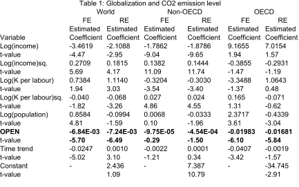
per capita CO2 emission level, Table 1 shows that the coefficient of openness is negative

for all three groups and statistically significant except Non-OECD country group. This

suggests that globalization help to reduce pollution in developed country not in

developing country. In case of CO2 emission intensity per dollar (Table 2) and relative

change of CO2 emission per capita (Table 3), the coefficients of openness are

significantly negative in OECD and the World but positive in Non-OECD country group.

Thus, unambiguously globalization helps developed countries to reduce emission (or

pollution) while it increases in under developed country. Table 2 and Table 3 point out

that globalization promotes to increase emission (pollution) intensity and relative change

of emission and thereby liberalization or openness hurts the environment of developing

country and improves the environment of developed country. Thus, these empirical

findings (Table 1 – 3) support the pollution haven hypothesis (PHH). This finding

support the earlier studies (Low and Yeats (1992), Agras and Chapman (1999) and Suri

intensive goods while less developed countries produce more and more

pollution-intensive goods.

However, conventional trade theory suggests that capital abundant countries

export the capital-intensive goods, (which is also energy intensive,) which increases

pollution in capital abundant country4. So, it seems that the PHH and FEH contradict.

Actually, the differences in environmental policy (PHH) and differences in factor

endowments (FEH) might interact and jointly may determine the comparative advantage

in trade. The possible interaction effects are incorporated in our last two equations i.e.,

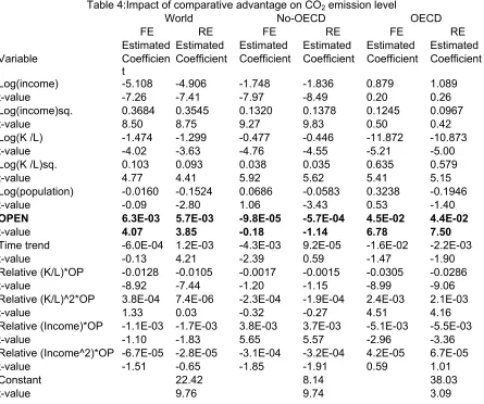
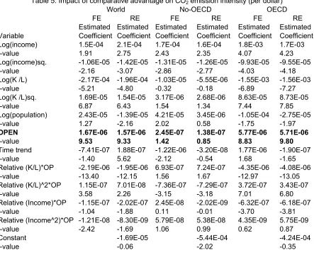
eq. (3)-(4). Now we present the estimates from our equations (3) – (4) allowing for the

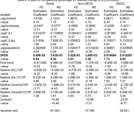
interaction of country characteristics with a measure of openness. Table 4, Table 5 and

Table 6 present the estimated results of the impact of comparative advantage (interaction

with country characteristics) on emission level, emission intensity and relative change of

emission, respectively. The results are dramatically changed. Table 4, Table 5 and Table

6 present that the coefficient of openness is positive and significant for all three measures

of pollution for all three groups, except negative and insignificant λ(coeff. Of openness)

for emission level in Non-OECD country group. It should be noted that adding the

country characteristics show to have made a large difference to the impact openness has

on CO2 emission. The signs of the coefficient of openness change dramatically opposing

the previous results (i.e., PHH) with high significant level. This result differs from the

findings of Antweiler et al. (2001), and Copeland and Taylor (20045). The interaction

terms with country characteristics are also highly significant. The interaction term on

4

Globalization helps to concentrate on the capital-intensive industry and thereby raising pollution. 5

openness and relative capital-labour ratio is negative and its square term is positive in

most of the cases except in Non-OECD for emission intensity (see Table 4 - 6). Now we

observe the interaction terms (on relative capital and openness) are negative and positive

for all three measures in the world and OECD. Therefore, if a country has sufficiently

high capital-labour ratio relative to the rest of the world, further openness makes this

country cleaner. Relatively rich and poor country would be cleaner and dirtier6,

respectively. This implies that rich capital abundant country diverts one part of their

capital and labour to produce clean and knowledge-based technology. The results of

interaction on openness and relative income are also similar to that of capital-labour ratio.

Net impact of globalization on emission depends on the relative strength of the factor

endowments and policy regulations. Globalization raises emission in the world while it

reduces emission marginally in OECD and increases in Non-OECD countries. These

empirical findings suggest that globalization increases the pollution, particularly CO2

emission, and thereby help to rise the global warming.

5. Conclusion

The aim of this paper is to explore whether globalization helps or hurts the

environment. Using panel data technique we examine the impacts of globalization on

pollution level, pollution intensity and relative change of pollution for the developed

(OECD) and developing (Non-OECD) country groups and the world as a whole. This

paper examines the factor endowment and pollution haven hypotheses that predict how

international trade affects the environment. In this study we use CO2 emission, which is

6

the mail culprit of the global warming, and observe that the impact of globalization on

environment heavily depends on the basic characteristics of a country and its dominating

comparative advantage. The empirical results suggest that globalization help developed

countries to reduce CO2 emission while developing countries to rise CO2 emission. Net

impact of globalization increases the global worming.

References

• Agras, J. and D. Chapman (1999): “A dynamic approach to the Environmental

Kuznets Curve hypothesis”, Ecological Economics 28(2), 267 - 277.

• Antweiler, W., B. R. Copeland and M. S. Taylor (2001): “Is Free Trade Good for the Environment?”, American Economic Review 91(4), 877 – 908.

• Baltagi, B. H. (1999): Econometric Analysis of Panel Data, John Wiley & Sons, New York.

• Bommer, Rolf (1999): “Environmental Policy and Industrial Competitiveness: The Pollution Haven Hypothesis Reconsidered”, Review of International Economics 7(2), 342 – 355.

• Brock, W. A. and M. S. Taylor (2004): “Economic Growth and the Environment: A

Review of Theory and Empirics”, NBER Working Paper 10854.

• Cole, M. A. (2004): “Trade, the pollution haven hypothesis and the environmental

Kuznets curve: examining the linkages”, Ecological Economics 48 (1), 71-81.

• Coondoo, D. and S. Dinda (2002): “Causality between income and emission: a country group-specific econometric analysis”, Ecological Economics 40 (3), 351 -367.

• Copeland, B. R., and M. S. Taylor (2004): “Trade, Growth and the Environment”,

Journal of Economic Literature XLII, 7 – 71.

• Copeland, B. R., and M. S. Taylor (1995): “Trade and environment: a partial synthesis”, American Journal of Agricultural Economics 77, 765 - 771.

• Dinda, S., and D. Coondoo (2006): “Income and Emission: A Panel Data based

Cointegration Analysis”, Ecological Economics 57(2), 167 - 181.

• Grossman, G. M. and A. B. Krueger (1991): “Environmental impacts of the North

American Free Trade Agreement”, NBER working paper 3914.

• Hettige, H., R. E. B. Lucas and D. Wheeler (1992): “The Toxic Intensity of Industrial Production: Global patterns, Trends and Trade Policy”, American Economic Review

82, 478 - 481.

• Hettige, H., M. Mani and D. Wheeler (2000): “Industrial pollution in economic

development: the environmental Kuznets curve revisited”, Journal of Development Economics 62, 445 - 476.

• Kuznets, Simon (1955): “Economic Growth and income inequality”, American Economic Review 45, 1 - 28.

• Liang, F. H., (2006): “Does Foreign Direct Investment Harm the Host Country’s

Environment? Evidence from China”, UC Berkeley, mimeo.

• Liddle, B. (2001): “Free trade and the environment-development system”, Ecological Economics 39, 21 – 36.

• Lopez, R. (1994): “The environment as a factor of production: the effects of economic growth and trade liberalization”, Journal of Environmental Economics and management 27, 163 - 184.

• Low, P. and A. Yeats (1992): “Do ‘dirty’ industries migrate?” In P. Low (ed.),

International Trade and environment., World Bank., Washington, D.C.

pollution: 1960 – 1988”, in P. Low (ed.) International Trade and the Environment, World Bank discussion paper 159, World Bank., Washington, D.C.

• Mani, M. and D. Wheeler (1998): “In search of pollution havens? Dirty industry in the world economy: 1960 – 1995”., Journal of Environment and Development 7(3), 215 - 247.

• Mukhopadhyay, K., Chakraborty, D. and Dietzenbacher, E., (2005): “Pollution Haven

and Factor Endowment Hypotheses Revisited: Evidence from India”, paper presented in the Fifth International Input-Output Conference at Renmin University in Beijing, China, during June 27 – July 1.

• Oak Ridge National Laboratory, CDIAC, Environmental Science Division, 1998, Estimates of global, regional and national CO2 emissions from fossil fuel burning,

cement manufacturing and gas flaring: 1755 – 1996, available at

http://www.cdiac.esd.ornl.gov/epubs/ndp030/global97.ems, (updated 2000).

• Rothman, D. S. (1998): Environmental Kuznets curve- real progress or passing the

buck?: A case for consumption-base approaches, Ecological Economics 25, 177-194.

• Summers, R. and A. Heston (1994): “Penn World Table (Version 5.6): An Expanded Set of International Comparisons:1950–1992”, NBER, PWT5.6, available at

http://www.nber.org/pwt5.6.

• Suri, V. and D. Chapman (1998): Economic growth, trade and the energy:

implications for the environmental Kuznets curve, Ecological Economics 25, 195 -208.

• Temurshoev, U., (2006): “Pollution Haven Hypothesis or Factor Endowment Hypothesis: Theory and Empirical Examination for the US and China”, CERGE-EI,

Working paper 292.

• Tisdell, C. (2001): “Globalisation and sustainability: environmental Kuznets curve

and the WTO”, Ecological Economics 39, 185 -196.

• Wheeler, D. (2000): “Racing to the Bottom? Foreign Investment and Air Pollution in

Developing Countries”, World Bank Development Research Group Working Paper

No. 2524.

Table 1: Globalization and CO2 emission level

World Non-OECD OECD

FE RE FE RE FE RE

Estimated Estimated Estimated Estimated Estimated Estimated Variable Coefficient Coefficient Coefficient Coefficient Coefficient Coefficient Log(income) -3.4619 -2.1088 -1.7862 -1.8786 9.1655 7.0154

t-value -4.47 -2.95 -9.04 -9.65 1.94 1.57

Log(income)sq. 0.2709 0.1815 0.1382 0.1444 -0.3855 -0.2931

t-value 5.69 4.17 11.09 11.74 -1.47 -1.19

Log(K per labour) 0.7384 1.1140 -0.3204 -0.3030 -3.3488 1.0643

t-value 1.94 3.03 -3.54 -3.40 -1.37 0.48

Log(K per labour)sq. -0.040 -0.068 0.027 0.024 0.165 -0.071

t-value -1.82 -3.26 4.86 4.55 1.31 -0.62

Log(population) 0.8584 -0.0994 0.0068 -0.0333 2.3717 -0.4339

t-value 4.81 -1.59 0.10 -1.96 3.61 -3.04

OPEN -6.84E-03 -7.24E-03 -9.75E-05 -4.54E-04 -0.01983 -0.01681

t-value -5.70 -6.49 -0.29 -1.50 -6.10 -5.84

Time trend -0.0247 0.0010 -0.0022 0.0001 -0.0407 -0.0019

t-value -5.02 3.10 -1.21 0.34 -3.42 -1.57

Constant - 2.436 - 7.387 - -34.745

t-value 1.09 10.79 -2.91

Table 2: Globalization and CO2 emission intensity (per dollar)

World Non-OECD OECD

FE RE FE RE FE RE

Estimated Estimated Estimated Estimated Estimated Estimated Variable Coefficient Coefficient Coefficient Coefficient Coefficient Coefficient Log(income) 4.1E-04 6.4E-04 2.4E-04 2.3E-04 2.9E-03 2.5E-03

t-value 4.37 7.38 3.87 3.71 5.72 5.19

Log(income)sq. -2.6E-05 -4.1E-05 -1.7E-05 -1.7E-05 -1.7E-04 -1.5E-04

t-value -4.49 -7.74 -4.46 -4.29 -5.95 -5.48

Log(K per labour) 1.3E-04 1.9E-04 2.6E-05 2.7E-05 -4.2E-04 -1.3E-05

t-value 2.71 4.22 0.91 0.98 -1.59 -0.05

Log(K per labour)sq. -5.5E-06 -1.0E-05 7.8E-07 5.0E-07 2.4E-05 2.7E-06

t-value -2.04 -4.04 0.45 0.29 1.76 0.21

Log(population) 1.5E-04 -7.5E-06 2.6E-05 1.6E-06 1.8E-04 -5.7E-05

t-value 6.83 -1.05 1.26 0.28 2.51 -4.09

OPEN -4.5E-07 -5.8E-07 3.3E-07 2.5E-07 -3.2E-06 -2.5E-06

t-value -3.06 -4.25 3.14 2.58 -9.18 -8.09

Time trend -4.2E-06 1.6E-07 -8.6E-07 -2.8E-08 -1.5E-06 -1.7E-07

t-value -6.92 4.55 -1.51 -0.46 -1.15 -1.42

Constant - -3.1E-03 - -9.0E-04 - -9.9E-03

Table 3: Globalization and Relative change of CO2 emission

World Non-OECD OECD

FE RE FE RE FE RE

Estimated Estimated Estimated Estimated Estimated Estimated Variable Coefficient Coefficient Coefficient Coefficient Coefficient Coefficient Log(income) 2.3184 3.2181 2.5481 2.4073 10.6059 9.5839

t-value 7.13 10.66 6.46 6.17 8.09 7.72

Log(income)sq. -0.0893 -0.1474 -0.1139 -0.1052 -0.5402 -0.4873

t-value -4.47 -8.02 -4.58 -4.27 -7.40 -7.12

Log(K per labour) 0.798 1.031 0.301 0.339 -1.422 0.120

t-value 4.99 6.65 1.67 1.90 -2.09 0.19

Log(K per labour)sq. -0.0340 -0.0536 0.0006 -0.0046 0.0688 -0.0117

t-value -3.70 -6.10 0.05 -0.42 1.97 -0.37

Log(population) 0.567 0.016 0.418 -0.006 0.972 -0.069

t-value 7.57 0.57 3.17 -0.17 5.33 -1.76

OPEN 9.3E-04 -7.7E-05 3.5E-03 2.3E-03 -4.4E-03 -3.4E-03

t-value 1.86 -0.16 5.27 3.77 -4.90 -4.21

Time trend -0.0165 0.0008 -0.0142 -0.0001 -0.0103 -0.0006

t-value -7.99 4.99 -3.92 -0.35 -3.10 -1.92

Constant -22.403 -16.068 -44.986

Table 4:Impact of comparative advantage on CO2 emission level

World No-OECD OECD

FE RE FE RE FE RE

Estimated Estimated Estimated Estimated Estimated Estimated Variable Coefficien

t

Coefficient Coefficient Coefficient Coefficient Coefficient

Log(income) -5.108 -4.906 -1.748 -1.836 0.879 1.089

t-value -7.26 -7.41 -7.97 -8.49 0.20 0.26

Log(income)sq. 0.3684 0.3545 0.1320 0.1378 0.1245 0.0967

t-value 8.50 8.75 9.27 9.83 0.50 0.42

Log(K /L) -1.474 -1.299 -0.477 -0.446 -11.872 -10.873

t-value -4.02 -3.63 -4.76 -4.55 -5.21 -5.00

Log(K /L)sq. 0.103 0.093 0.038 0.035 0.635 0.579

t-value 4.77 4.41 5.92 5.62 5.41 5.15

Log(population) -0.0160 -0.1524 0.0686 -0.0583 0.3238 -0.1946

t-value -0.09 -2.80 1.06 -3.43 0.53 -1.40

OPEN 6.3E-03 5.7E-03 -9.8E-05 -5.7E-04 4.5E-02 4.4E-02

t-value 4.07 3.85 -0.18 -1.14 6.78 7.50

Time trend -6.0E-04 1.2E-03 -4.3E-03 9.2E-05 -1.6E-02 -2.2E-03

t-value -0.13 4.21 -2.39 0.59 -1.47 -1.90

Relative (K/L)*OP -0.0128 -0.0105 -0.0017 -0.0015 -0.0305 -0.0286

t-value -8.92 -7.44 -1.20 -1.15 -8.99 -9.06

Relative (K/L)^2*OP 3.8E-04 7.4E-06 -2.3E-04 -1.9E-04 2.4E-03 2.1E-03

t-value 1.33 0.03 -0.32 -0.27 4.51 4.16

Relative (Income)*OP -1.1E-03 -1.7E-03 3.8E-03 3.7E-03 -5.1E-03 -5.5E-03

t-value -1.10 -1.83 5.65 5.57 -2.96 -3.36

Relative (Income^2)*OP -6.7E-05 -2.8E-05 -3.1E-04 -3.2E-04 4.2E-05 6.7E-05

t-value -1.51 -0.65 -1.85 -1.91 0.59 1.01

Constant 22.42 8.14 38.03

Table 5: Impact of comparative advantage on CO2 emission intensity (per dollar)

World No-OECD OECD

FE RE FE RE FE RE

Estimated Estimated Estimated Estimated Estimated Estimated Variable Coefficient Coefficient Coefficient Coefficient Coefficient Coefficient Log(income) 1.5E-04 2.1E-04 1.7E-04 1.6E-04 1.8E-03 1.7E-03

t-value 1.91 2.75 2.43 2.35 4.07 4.23

Log(income)sq. -1.06E-05 -1.42E-05 -1.31E-05 -1.26E-05 -9.93E-05 -9.55E-05

t-value -2.16 -3.07 -2.86 -2.77 -4.03 -4.18

Log(K /L) -2.17E-04 -1.96E-04 -1.03E-05 -5.55E-06 -1.55E-03 -1.56E-03

t-value -5.21 -4.80 -0.32 -0.18 -6.89 -7.27

Log(K /L)sq. 1.69E-05 1.54E-05 3.17E-06 2.68E-06 8.63E-05 8.73E-05

t-value 6.87 6.43 1.54 1.34 7.44 7.85

Log(population) 2.43E-05 -1.39E-05 4.21E-05 3.45E-06 -1.05E-04 -2.75E-05

t-value 1.27 -2.16 2.02 0.58 -1.75 -1.97

OPEN 1.67E-06 1.57E-06 2.45E-07 1.38E-07 5.77E-06 5.71E-06

t-value 9.53 9.33 1.42 0.85 8.83 9.80

Time trend -7.41E-07 1.88E-07 -1.22E-06 -3.20E-08 1.77E-06 -1.90E-07

t-value -1.40 5.62 -2.12 -0.54 1.68 -1.65

Relative (K/L)*OP -2.19E-06 -1.95E-06 6.93E-07 7.24E-07 -4.35E-06 -4.08E-06

t-value -13.40 -12.15 1.56 1.67 -12.97 -13.05

Relative (K/L)^2*OP 1.15E-07 7.01E-08 -7.36E-07 -7.29E-07 3.72E-07 3.43E-07

t-value 3.58 2.26 -3.15 -3.18 7.01 6.80

Relative (Income)*OP -1.15E-07 -2.02E-07 2.45E-08 -2.02E-09 -6.32E-07 -6.18E-07

t-value -1.04 -1.88 0.11 -0.01 -3.70 -3.81

Relative (Income^2)*OP -1.21E-08 -8.30E-09 5.79E-08 5.38E-08 4.35E-09 5.75E-09

t-value -2.42 -1.69 1.06 0.99 0.62 0.87

Constant -1.69E-05 -5.44E-04 -4.24E-04

Table 6: Impact of comparative advantage on relative change of CO2 emission

World Non-OECD OECD

FE RE FE RE FE RE

Estimated Estimated Estimated Estimated Estimated Estimated Variable Coefficient Coefficient Coefficient Coefficient Coefficient Coefficient Log(income) 1.6156 2.1244 1.8679 1.8599 6.9611 6.8833

t-value 5.15 7.15 4.15 4.16 5.43 5.74

Log(income)sq. -0.0447 -0.0777 -0.0692 -0.0695 -0.3226 -0.3211

t-value -2.31 -4.27 -2.37 -2.40 -4.50 -4.84

Log(K /L) 0.014237 0.118808 -0.064421 0.056897 -2.87362 -2.45619

t-value 0.09 0.74 -0.31 0.28 -4.38 -3.93

Log(K /L)sq. 0.01836 7.89E-03 0.026822 0.015461 0.155571 0.133333

t-value 1.90 0.84 2.04 1.21 4.61 4.12

Log(population) 0.362689 7.57E-03 0.526417 -0.014234 0.39951 0.020658

t-value 4.83 0.28 3.96 -0.36 2.29 0.52

OPEN 6.49E-03 5.63E-03 5.52E-03 3.60E-03 0.014684 0.015287

t-value 9.44 8.44 5.01 3.48 7.73 9.05

Time trend -0.011084 8.36E-04 -0.017536 -1.31E-04 -5.94E-03 -7.68E-04

t-value -5.33 5.43 -4.79 -0.32 -1.93 -2.37

Relative (K/L)*OP -5.92E-03 -5.32E-03 -4.77E-03 -2.99E-03 -9.73E-03 -9.70E-03

t-value -9.22 -8.39 -1.68 -1.08 -9.99 -10.68

Relative (K/L)^2*OP 6.23E-04 4.28E-04 2.88E-04 -2.59E-04 1.08E-03 1.06E-03

t-value 4.96 3.49 0.19 -0.18 7.02 7.21

Relative (Income)*OP -1.62E-03 -1.88E-03 8.21E-04 5.53E-04 -2.54E-03 -2.72E-03

t-value -3.71 -4.43 0.60 0.41 -5.11 -5.77

Relative (Income^2)*OP 2.69E-05 3.12E-05 3.24E-04 2.51E-04 5.62E-05 6.64E-05

t-value 1.36 1.61 0.93 0.73 2.77 3.45

Constant -14.98 -12.98 -23.97

t-value -14.48 -7.51 -6.77

Clean goods

P Figure 1: Pollution Haven Hypothesis

B

A

Q

C

D

O P Q Dirty goods