Face Detection using Color based
Segmentation and Edge Detection
Jagdish Prasad Goswami
M.Tech Scholar Department of CSE
Mewar University Chittorgarh, Rajasthan
Preetam Kr. Chourasiya
M.Tech Scholar Department of ECE RKDF Inst. Of Tech.
Bhopal, MP
Nipendra Singh Chauhan
M.Tech Scholar Department of CSE
Manav Bharti University, HP
ABSTRACT
The increasing use of computer vision in security in place of humans led many to research the problem of face detection in images. The problem is not a petty one as the classification of a human face proves to challenging. Despite the many variations of a human face, features can still be found, given a certain context, which will uniquely identify a face. Early face-detection algorithms focused on the detection of frontal human faces, whereas this paper attempt to solve the more general and difficult problem of multi-view face detection. Face detection involves many research challenges such as scale, rotation, and pose and illumination variation. The techniques used for face detection have been researched for years and much progress has been suggested in literature. This paper proposes a new technique for detecting faces in color images using color modeland edge detection. Face detection is used in as a part of a facial recognition system. It is also used in human computer interface, image database management and video surveillance. The results of this technique show that the proposed algorithm is good enough to detect the human face taken through video with accuracy. This paper is achieving high detection speed, high detection accuracy and reduces the false detecting rate.
Keywords
Face detection, Color segmentation, Color model, Edge detection, Canny edge detector.
1.
INTRODUCTION
Face detection is the method of discovering all possible faces at different locations with different sizes in a given image. Face detection locates and segments face regions in cluttered images. It has various applications in areas like security control systems, surveillance, content-based image retrieval, intelligent human computer interfaces and video conferencing [1] [2]. The system segments faces in cluttered images face. As a visual frontend processor, a face detection system should also be able to achieve the task regardless of illumination, orientation, and camera distance [3]. A system that performs face detection or recognition will find many applications such as surveillance cameras and security control systems. Face detection is used in many places now days especially the websites hosting images like photobucket, facebook and picassa. The automatically tagging feature adds a new dimension to sharing pictures among the people who are in the picture and also gives the idea to other people about who the person is in the image. This paper implemented a pretty
simple but very effective face detection algorithm which takes human skin color into account [4].
Face detection is the first step of face recognition as it automatically detects a face from a complex background to which the face recognition algorithm can be applied. But detection itself involves many complexities such as background, poses, illumination etc. Face detection rate and the number of false positives are important factors in evaluating face detection systems. Face detection rate is the ratio between the number of faces correctly detected by the system and the actual number of faces in the image [5] [6]. Most face detection systems attempt to extract a fraction of the full face, thereby eliminating most of the background and other areas of an individual's head such as hair that are not necessary for the face recognition task [7]. With static images, this is usually done by running a 'window' across the image. The face detection method then judges if a face is present inside the window. Unfortunately, with static images there is a very large search space of possible locations of a face in an image. Faces may be 21 large or small and be positioned anywhere from the upper left to the lower right of the image.
The development of the feature-based approach can be further divided into three areas. Given a typical face detection problem in locating a face in a cluttered scene, low-level analysis first deals with the segmentation of visual features using pixel properties such as color and gray-scale. Due to low-level nature, features generated by this analysis are indistinct. In feature analysis, visual features are organized into a more global concept of face and facial features using information of face geometry. Through feature analysis, feature ambiguities are reduced and locations of the face and facial features are determined [8].
This paper is categorized into six sections. The first section gives the introduction of face detection. The second section define the color segmentation, in which there are different types of color spaces like CIEXYZ, HSV, YCbCr, YUV, YCoCg color space. The third section deals with edge detection, which use canny edge detector to detect the edge. The fourth section draws the block diagram of design approach. The fifth section concludes conclusion and future scope and last sixth section end with references.
2.
COLOR SEGMENTATION
skin and non-skin classes while decreasing the separability among skin tones [3]. Hopefully it will bring robust performance under varying illumination conditions. However, there are many color spaces to choose from and a large number of metrics to judge whether they are effective. Segmentation techniques locate objects consisting of pixels having something in common. Commonly this means that pixels with almost the same intensity values are grouped together, or pixels with the same color code. There are techniques for finding for instance objects with convex objects, closed contours and the boundaries of an object. The segmentation principle states that the first step in processing a pixel should be to segment the local region encompassing that pixel. This provides a snapshot of the local structural features of the image, with the signal clearly separated from the noise. It is hoped that the identified structural information could be used to implement many image processing tasks including [10].
This paper present five color spaces that are:
CIEXYZ
HSV and HLS
YCbCr
YUV
YCoCg
2.1
CIEXYZ Color Space
[image:2.595.61.276.495.679.2]The CIEXYZ color space is developed by the CIE (Commission Internationale de l’Eclairage) is an international standard. This color space is based on three hypothetical primaries X, Y and Z. All the visible colors can be represented by X, Y and Z components positive values. The primaries in CIEXYZ color space are hypothetical because they do not contain any real light wavelengths. Y primary is used to define to match closely to luminance, while X and Z primaries are used to define the color information. The major advantage of the XYZ color model is that this space is completely independent of device [11]. The block position RGB colors in the CIEXYZ color space is shown in Figure.
Figure 1: CIEXYZ Color Space
The following basic equations to convert RGB color space to XYZ color space and XYZ color space to RGB color space.
X = 0.412453*R + 0.35758 *G + 0.180423*B
Y = 0.212671*R + 0.71516 *G + 0.072169*B
Z = 0.019334*R + 0.119193*G + 0.950227*B
R = 3.240479 * X - 1.53715 * Y - 0.498535 * Z
G = -0.969256 * X + 1.875991 * Y + 0.041556 * Z
B = 0.055648 * X - 0.204043 * Y + 1.057311 * Z
2.2
HSV and HLS Color Space
The HSV (hue, saturation, value) and HLS (hue, lightness, saturation) color models were designed to approximate the way humans perceive and were developed to be more intuitive in manipulating with color and interpret color.
Hue defines the color itself. The values for the hue axis vary from 0 to 360 beginning and ending with red and running throughout green, blue and all mediator colors. Saturation indicates that the degree to which the hue differs from an impartial gray. The values run from 0, which means no color saturation and 1, which is the whole saturation of a given hue at a given illumination. The value HLS or value HSV indicates the illumination level. Both vary from 1 (white, full illumination) to 0 (black, no light). The differences between them is that maximum saturation (S=1) of hue in the HLS color space with lightness L=0.5 and at value V=1 in the HSV color space.
2.3
YCbCr Color Space
The YCbCr color space is widely used for various applications. In this format, luminance information is stored as a single component (Y), and chrominance information is stored as two color-difference components (Cb and Cr). Cb component represents the difference between the blue component and a reference value. Cr component represents the difference between the red component and a reference value. YCbCr value can be double precision, but the color space is typically well suited to 8 bit data. For 8 bit images, the data range for Y is [16, 235], and the range for Cb and Cr is [16, 240]. YCbCr leaves room at the top and bottom of the full 8 bit range so that additional (nonimage) information can be included in a video stream [12].
The following basic equations to convert RGB and YCbCr are
Y = (77/256)R + (150/256)G + (29/256)B
Cb = ‐(44/256)R ‐ (87/256)G + (131/256)B + 128
Cr = (131/256)R ‐ (110/256)G ‐ (21/256)B + 128
R = 1.164*(Y-16) + 1.596*(Cr-128)
G = 1.164*(Y-16) - 0.813*(Cr-128) - 0.392*(Cb-128)
B = 1.164*(Y-16) + 2.017*(Cb-128)
Figure 2: YCbCr Color Space
2.4
YUV Color Space
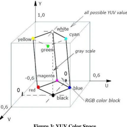
The YUV color space is the recoding of RGB for downward compatibility with black-and white television and for transmission efficiency (minimum bandwidth). The YUV color space is generate from the RGB space. It comprises the luminance (Y) component and two color difference (U, V) components. The luminance value can be calculated as a weighted sum of red, green and blue components of color. The color difference or components, chrominance are formed by subtracting luminance from red and blue.
The principal advantage of the YUV color model in image processing is color information and decoupling of luminance. The significance of this decoupling is that the luminance component of an image can be processed without affecting its color components. YUV were used for a specific analog encoding of color information in television systems.
Figure 3: YUV Color Space
There are several combinations of YUV color values from nominal ranges that result in invalid RGB values, because the possible RGB colors engage only piece of the YUV color space limited by these ranges. Below figure shows the valid
color block in the YUV color space that corresponds to the RGB color cube RGB values are normalized to [0, 1]). The YUV notation means that the components are produce from gamma-corrected RGB. Weighted sum of these non-linear components of color space forms a signal representative of luminance that is called luma component Y.
The following basic equation to convert between gamma-corrected RGB and YUV models:
R = Y + 1.4075 * (V - 128)
G = Y - 0.3455 * (U - 128) - (0.7169 * (V - 128))
B = Y + 1.7790 * (U - 128)
Y = R * 0.299000 + G * 0.587000 + B * 0.114000
U = R * -0.168736 + G * -0.331264 + B * 0.500000 + 128
V = R * 0 .500000 + G * -0.418688 + B * -.081312 + 128
2.5
YCoCg Color Space
[image:3.595.317.554.370.568.2]The YCoCg color model was developed to increase the effectiveness of the image compression. This color model comprises the luminance (Y) and two color difference components (Co - offset orange, Cg - offset green).
Figure 4: YCoCg Color Space
There are following simple basic equations to convert between RGB and YCoCg:
Y = R/4 + G/2 + B/4
Co = R/2 - B/2
Cg = -R/4 + G/2 - B/4
R = Y + Co - Cg
G = Y + Cg
[image:3.595.57.272.494.710.2]A variation of this type of color space which is called YCoCg color space enables transformation reversibility with smaller dynamic range requirements than does YCoCg. The possible value of RGB colors engage only part of the YCoCg color space limited by the nominal ranges, therefore there are several combinations of YCoCg that result in invalid RGB values.
3.
EDGE DETECTION
After an image is segmented using CIEXYZ and YCbCr color model, apply edge detection method. Edge detection is an important preprocessing step in various computer vision algorithms [13] [14]. Within this paper we implement the Canny Edge Detector method.
3.1
Canny Edge detector
The Canny edge detection algorithm is known to many as the optimal edge detector. Canny edge detector were to enhance the many edge detectors already out at the time started work [15] [16].
Step1: The first step of edge detection is to filter out any noise in the original image before trying to locate and detect any edges. The Gaussian filter can be completed by a simple mask, it is used completely in the Canny edge detector. Once a proper mask has been determined, the Gaussian smoothing can be performed by standard convolution methods. A convolution mask is usually much lesser than the real image. Thus, the mask is slid over the image, manipulating a square of pixels at a instance. The large width of the Gaussian mask, the lower is the sensitivity of detector to noise. The localization error in the detected edges also increases a little as the Gaussian width is increased. The Gaussian mask is shown below.
Figure 5: Discrete Approximation to Gaussian Function
[image:4.595.58.237.406.539.2]Step 2: After eliminating the noise and smoothing the image, the next step is to find the edge strength by taking the gradient of the image. The Sobel operator operates a 2-D spatial gradient measurement on an image. Then, the estimated absolute gradient magnitude can be found at each point. The Sobel operator take a couple of 3x3 convolution masks, one approximating the gradient in the x-direction (columns) and the other estimating the gradient in the y-direction (rows). They are shown below:
Figure 6: Approximated Gradient
[image:4.595.331.548.613.705.2]The edge strength or magnitude of the gradient is then approximated using the formula:
|G| = |Gx| + |Gy|
Step 3: Finding the edge direction is slight once the gradient in the x and y directions are known. However, we will produce an error whenever sum X is equal to zero. So in the code there has to be a constraint set whenever this takes place. Whenever the gradient of edge in the x direction is equal to zero, the edge direction has to be equal to 0 degrees or 90 degrees, depending on what the value of the gradient in the y-direction. If Gy has a value of zero, the edge direction will equal to 0 degrees, otherwise the edge direction will equal to 90 degrees [17]. The formula for calculating the edge direction is as:
theta = invtan (Gy / Gx)
Step 4: After calculating the edge direction, the next step is to relate the edge direction to a direction that can be traced in an image. As a result if the pixels of a 5x5 image are aligned as follows:
x x x x x x x x x x x x a x x x x x x x x x x x x
Then, it can be seen by looking at pixel "a", there are only four possible directions when describing the surrounding pixels 0 degrees (in the horizontal direction), 45 degrees (along the positive diagonal), 90 degrees (in the vertical direction), or 135 degrees (along the negative diagonal). So now the edge direction has to be resolved into one of these four directions depending on which direction it is closest to. Assume of this as taking a semi circle and dividing it into 5 regions.
Figure 7: Edge Direction Diagram
within the blue range (67.5 to 112.5 degrees) is set to 90 degrees. Finally any edge direction falling within the red range (112.5 to 157.5 degrees) is set to 135 degrees.
Step 5: After the edge directions are finding, nonmaximum suppression now has to be applied. A Nonmaximum suppression is used to trace along the edge in the edge direction and suppress any pixel value (sets it equal to 0) 0 so that is not considered to be an edge. This will produce a thin line in the output image.
Step 6: Finally, hysteresis is used as a means of eliminating streaking. The streaking is the breaking up of an edge contour caused by the operator output fluctuating above and below the threshold. If a single threshold value, T1 is applied to an image, and an edge has an average strength of edge is equal to T1, then due to noise, there will be instances where the edge dips below the threshold. Equally it will also expand above the threshold making an edge look like a dashed line. To avoid this type of problem, hysteresis uses two thresholds, a low and a high. Any pixel in the image that has a value greater than T1 is presumed to be an edge pixel, and is marked such as immediately. Then, any pixels that are connected to this edge pixel and that have a value greater than T2 are also selected as edge pixels [18].
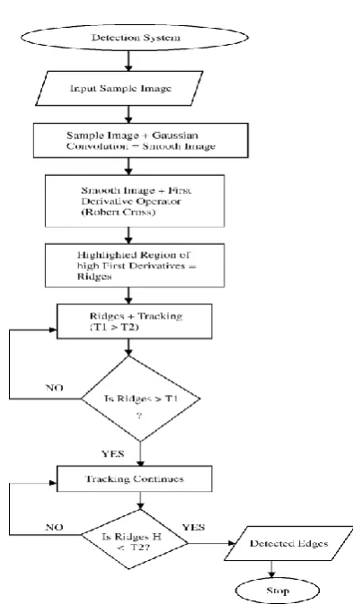
[image:5.595.65.262.326.668.2]4.
DESIGN APPROACH
Figure 8: Block diagram of design approach
5.
CONCLUSION AND FUTURE SCOPE
The main contribution of this paper is to propose a method to construct a simple and fast face detection system. Initially the images are enhanced by contrast adjustment and noise removal. Then the images are divided into number of blocks to extract the rectangle features. The feature values are calculated or the block is considered based on a novel edge tracking algorithm. This paper proposes an algorithm with good accuracy and running time for face detection based on Canny Edge Detector algorithm. Though there are some cases of false positives, the overall performance of the proposed algorithm is quite satisfactory. We can implement this technique in real time application. We can also implement this technique with hardware.
6.
REFERENCES
[1] Chandrashekar M Beedimani, “Automated face detection in color images using skin region and adaptive template matching”, IJCER Journal.
[2] Ming-Hsuan Yang et.al. “Detecting faces in Images: a survey”, IEEE transaction on Pattern analysis and machine intelligene, vol. 24, no.1 2002.
[3] Sanjay singh et.al, “A robust skin color based face detection algorithm”, Tamkang Journal of Science and Engineering vol.6, no.4,pp227-234, 2003.
[4] Henry A. Rowley, Shumeet Baluja, and Takeo Kanade. “Neural network based face detection”, IEEE Transactions on Pattern Analysis and Machine Intellig ence, 20(I), pp.23-38, 1998.
[5] Mohamed A. Berbar, Hamdy M. Kelash, and Amany A. Kandeel, “Face and Facial Features Detection in Color Images” Proceedings of the Geometric Modeling and Imaging New Trends (GMAI'06).
[6] J. Chen, C. M. Taskiran, A. Albiol, C. A. Bouman, and E. J. Delp, “Vibe: A video indexing and browsing environment,” in IEEE- SPlE Conference on Multirnedia Storage and Archiving Systems lV, Boston (USA), September 1999.
[7] M. Yagi and T. Shibata, .Human-Perception-Like Image Recognition System Based on the Associative Processor Architecture,. in the Proc. of 11th European Signal Processing Conference (EUSIPCO 2002), pp. 103 - I-106, Sep. 2002.
[8] Lalendra Sumitha Balasuriya, “Frontal View Human Face Detection and Recognition” University of Colombo Sri Lanka May 2000.
[9] Mohammad Mohmmad Fiuzy, Khosro Foad Rezaei, Javad Mohammad Haddadnia, “A Novel Approach For Segmentation Special Region In An Image”, MALJESI Journal of Multimedia Processing.
[10]T, Agui, Y. Kokubo, H. Nagashi, and T.Nagao, “Extraction of face recognition from monochromatic photographs using neural networks,” Proc. 2nd
Int’l Conf. Automation, Robotics, and Computer Vision, vol.1, pp. 18.81-18.8.5, 1992.
[11]Abhishek Gudipalli, Dr.Ramashri Tirumala, “Comprehensive Infrared Image Edge Detection Algorithm” International Journal of Image Processing (IJIP), Volume (6) : Issue (5) : 2012 .
[13]V. Torre and T. A. Poggio. “On edge detection”. IEEE Trans. Pattern Anal. Machine Intell., vol. PAMI-8, no.2, pp. 187-163, Mar. 1986.
[14]Y. Suzuki and T. Shibata, .Multiple-Clue Face Detection Algorithm Using Edge-Based Feature Vectors, accepted for presentation in IEEE International Conference on Acoustics, Speech, and Signal Processing (ICASSP 2004), May 2004.
[15]J. Canny. “Finding edges and lines in image”. Master’s thesis, MIT, 1983.
[16]M. Turk and A. Pentland, “Eigenfaces for recognition,” J. of Cognitive Neuroscience, vol.3, no. 1, pp. 71-86, 1991.
[17]Harshlata Vishwakarma, S.K.Katiyar, “Comparative Study of Edge Detection Algorithms on the remote sensing images Using matlab”, (IJAER) 2011, Vol. No. 2, Issue No. VI.\