Decreasing of Oil Extraction: Consumption behavior along transition paths

Munich Personal RePEc Archive

Decreasing of Oil Extraction:

Consumption behavior along transition

paths

Bazhanov, Andrei

8 October 2006

Online at

https://mpra.ub.uni-muenchen.de/469/

Decreasing of Oil Extraction: Consumption Behavior

Along Transition Paths

Andrei V. Bazhanov

October 08, 2006

∗_{Institute of Mathematics and Computer Science, Far Eastern National University, Vladivostok, Russia,}

e-mail: [email protected] or Department of Economics, Queen’s University, Kingston, ON K7L 3N6, Canada, phone: 1-(613)-533-2270, fax: 1-(613)-533-6668, e-mail: [email protected]

†_{Thanks to the Good Family Visiting Faculty Research Fellowship for}

financial support.

Abstract A normative analysis of the problem of optimal extraction of a non-renewable resource is considered. The economy depends on the essential non-renewable resource and the rate of the resource extraction increases over time. At some instant the government gradu-ally switches to a sustainable (in sense of non-decreasing consumption over time) pattern of the resource extraction. Different approaches are offered for the construction some curves of switching to decreasing paths of the resource depletion. Consumption paths have diverse be-havior patterns along these curves, including a path of unlimited growth. A new approach to the Rawlsian maximin criterion which allows for growth of consumption is offered.

Keywords Non-renewable resource · Intergenerational justice · Hartwick rule · Optimal path of extraction· Generalized Rawlsian criterion

1

Introduction

Theories are developing, governments are changing, and the criteria for the optimality of growth

can change from time to time. Wassily Leontief [27] described the dynamic inconsistency of

economic growth as follows: “...while each step, being determined by a conscious act of choice,

satisfies certain maximizing conditions, ... sequence as a whole does not. Its path can be

com-pared to the course of a dog running across a field toward his master, while the master walks

along the road. The dog’s path will usually describe a gentle arc, while the fastest way of joining

his master would be to run along a straight, properly aimed intercepting line”. In a number

of applications we present examples, for which we will observe “regime shifts” where we must

switch to a different path which is optimal according to new and different criteria or to diff

er-ent constraints. The problem offinding the optimal transition paths is standard in highway or

railroad construction and in other engineering applications (see, e.g., [22]). The problem also is

associated with so-called transition economics, as in [5], “...excess speed of closure” the public

enterprises for developing private sector “...may slow down transition because of output

con-traction effects”. And of course the construction of a transition path toward a sustainable path

is a concern of resource and environmental economics. For example, C. Fisher, C. Withagen,

and M. Toman [11] analyze a simple model which captures the main effects of the properties of

a transition path from “dirty” to “clean” (but more costly) technology. W.D. Nordhaus in his

works (see, e.g., [34]) considers a problem of optimal (in sense of utilitarian criterion) transition

to economy with less emission of greenhouse gases for the case of a Cobb-Douglas aggregate

technology. K. Farmer and R.Wendner [10] consider responses in a general two-sector model to

qualitatively different behavior (damped oscillation besides overshooting) for the model with

heterogeneous capital in comparison with the case of homogenous capital.

We are going to consider the problem of transition path construction for a case of changing

the growth path for world oil extraction for the Solow [43] model. Assume that we are not sure

if it is possible to find perfect substitutes for non-renewable resource use and come up with

alternative technologies during the period of the resource abundance. Then we must consider

the problem of construction the optimal resource extraction path from the point of view of

intergenerational justice. We show the existence of such a path in an example drawn from the

class of rational functions. In the future we are going to examine when it might be appropriate

to use such kind of curves as a way of switching smoothly to a sustainable extraction path (for

example, Hartwick’s curve). The aim of this paper is to examine consumption behavior along

the transition path itself. The main result (Proposition 2) shows that depending on parameters

of the path, consumption can decline to zero in finite time, asymptotically approach a

non-negative constant, or grow to infinity. The second case we argue is “asymptotically optimal” in

sense of Rawlsian maximin principle. There have been numerous attempts to reconcile Rawls’s

idea of supporting the least advantaged with the possibility of economic growth. Also there are

other criteria which imply different patterns of consumption growth as the optimal behavior1_.

We present a new modification of Rawlsian criterion (Generalized Rawlsian Criterion, GRC)

which implies a different interpretation of the “relevant social positions” for the comparison of

persons or generations, and as a result implies growth of consumption. The main idea does

not contradict various versions of the maximin criterion for intergenerational problems and we

1_{Different approaches to reconcile Rawls’ principle with economic growth can be found, e.g., in [1], [6], [15],}

can deal with overlapping generations or maximin in combination with the utilitarian criterion

and possibly other desiderata. The basic assumption of our approach postulates that utility

must depend not only on a current vector of static indicators of consumption but also on the

prehistory (derivative) of individual consumption. History is involved in the personal estimation

of an individual’s consumption level. This postulate can be applied either to problems of

intra-or intergenerational justice and so apparently it can help to solve the anomalous situation,

namely when very attractive and plausible principles can not be extended (as Rawls confirms

by himself [38], p.291) to intertemporal situations. We show with simple examples that

GRC-optimal consumption can exhibit limited growth (or limited decline) and unlimited growth

depending on the properties of the utility function. Thus, in general, transition paths of

essential resource extraction can be adjusted to different optimality criteria but the constraints

represented by difficulties in changing from oil-based technologies and from existing patterns

of saving do not allow the system to switch rapidly. Since we do not know the estimations of

parameters of such constraints, we do not consider them in our examples.

The social planner solves the Gray-Hotelling problem [13],[19] of maximization of the total

utility from the resource use during the finite period T of the resource existence:

T

0

U(r(t))dt_→max

r(t) .

For the case of the resource essential to production Solow [43] considered Rawlsian justice

principle for the resource allocation between generations as a limiting special case of utilitarian

criterion:

max

r(t) t∈min(0,∞)U(r(t)),

John Hartwick [17] showed the savings for the Solow [43] model must involve investing

current exhaustible resource returns in reproducible capital in order to maintain constant per

capita consumption over time. We review this for the case of a Cobb-Douglas technology. For

the case with zero population growth, no capital depreciation, no technological progress, and

zero extraction cost, we have output q = f(k, r) = kα_rβ _{where k is produced capital, r}

-current resource use, r =₋S, S˙ - resource stock, α, β _∈ (0,1) are constants. Prices of capital

and the resource are fk = α_kq, fr = βq_r. Per capita consumption is c = q−k.˙ The Hartwick

savings rule implies c=q₋rfr or, substituting forfr, c=q(1−β), which means that instead

of c˙= 0 we can checkq˙= 0.

From Hotelling rule fr_fr˙ =fk we have αβ_kq+ _rr˙(β−1) =fk =αq_k which in turn yields

˙

r r =−

αq

k . (1)

Then

˙

q q =α

˙

k k +β

˙

r r =β(

αq k +

˙

r

r) = 0, (2)

which means that we really haveq˙=c˙= 0.

Since from (2) q =const and then rfr =βq =const, we have k˙ =βq =const for deriving

k(t) and we have (1) forr(t). We can find two constants of integration k0 for k(t) = k0 +βqt

and the constant of equation

˙

r r =−

1

k0

αq +

β αt

using initial conditions r(0) = r0 and s(0) = s0, where s0 is the given resource stock which

must be used for production over infinite time: s0 = ₀∞r(t)dt. Then we have

r(t) =r0 1 +

r0β

s0(α−β)

t

−αβ

where α>β (Solow condition) and

˙

r(t) =₋¨s(t) =₋ αr

2 0

s0(α−β)

1 + r0β s0(α−β)

t

−(α+ββ)

. (4)

Since we assume that our economy depends on the resource essentially, we obtain path

r(t), asymptotically approaching zero and the path of extraction changes r(t)˙ (or negative

acceleration of stock s(t) diminishing) also approaching zero, but starting from the negative

valuer˙0 =− αr

2 0

s0(α−β).

2

Assuming that our economy has some “additional” savings, besides resource rent, it is

possible to relax the assumption of zero population growth (as in J. Stiglitz [44] and G. Asheim,

W. Buchholz, J. Hartwick, T. Mitra, and C. Withagen [3] papers), or zero capital depreciation.

But in any case, if we assume, that

1) economy at every instant of time depends on resource (even if we gradually introduce

substituting technologies and this dependence asymptotically approaches zero), and

2) we really want to maintain nondecreasing per capita consumption,

then rate of extraction r(t) must tend to zero.

Capital - resource substitution is a fundamental topic in energy economics and there are

some empirical evidences (see, e.g., [33], [36]) which can support the assumption that the

elasticity of substitution between natural resources and capital exceeds unity. This implies

that resource can be inessential. Though other investigations (e.g., [12], [30], and partly in

[16]) show that energy and capital are rather strong complements than substitutes (elasticity

is less than unity) and some researches find that this value is rather close to unity (e.g., [14],

2_{Path (3), asymptotically approaching zero, is necessary, but not sufficient condition of following Hartwick}

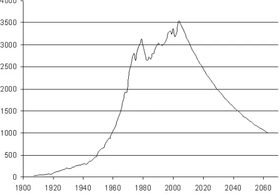
Figure 1: World oil extraction (mln.t./year)

[36]). In any case empirical evidences are not a proof and as P. Dasgupta and G. Heal noted

“Past evidence may not be a good guide for judging substitution possibilities for large values of

k/r”([7], p. 207). And so, we can assume that for the world economy oil is essential, especially

taking into account that no adequate immediate substitutes are available for transportation

fuels, a main area of oil use (see, e.g., [18], [31]). However, as we can see, for example, from oil

extraction data in December issues of Oil and Gas Journal, rates of extraction are in fact both

growing on the world level (see Fig. 1) and for the leading oil producers, not declining.

Assume that the government of our economy after period of oil-rent consumption and

grow-ing rate of extraction decided to conform to the intergenerational justice principle and switch

at t0 to some sustainable path of saving, e.g., to the Hartwick rule. An example with α = 0.3

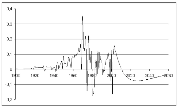
andβ = 0.05gives us behavior of r(t) andr(t)˙ for world oil extraction in Fig. 2 and Fig. 3.

An abrupt switch to the Hartwick rule means that people in oil-producing countries must

re-Figure 2: Historical data and Hartwick curve

structure their living style. Moreover, countries must instantly reorganize their economies,

because of the sharp decrease of consumption, which in turn leads to a decrease in production,

a possible increase in unemployment, and a further decrease of demand and so on. Thus, for

an economy not following the Hartwick rule, the sudden invocation of intergenerational justice

creates the dilemma of choosing between two awkward futures: diminishing consumption to zero

in the future because of the inevitable and increasing shortage of essential exhaustible resources

or diminishing consumption to a sustainable level right from the moment of switching to the

Hartwick rule.

Solow’s model implies that oil-rent is invested from the very beginning and that there is

no time gap between the moment of oil extraction and correspondent increase of reproducible

capital according to the Hartwick rule. We can consider it as an adequate model if we assume

that reproducible capital is a fund of some high-return securities and oil profit can be instantly

invested in some shares or bonds. But suppose that money bills are not able to substitute

gasoline in engines of our cars when we have shortage of oil. And the shortage will be the

inevitable result of growing demand because of economic growth and decreasing, according to

(3), supply of oil. It means, that in order to sustain non-decreasing output with the same

struc-ture, we must invest at least part of oil profit into development of oil-substituting technologies.

In other words, we must create an “anti-oil market” with the oil rent. And under this

assump-tion the model of instant investment can not be really adequate because of the difficulties of

a rapid re-structuring. Historical examples show that the development and the introduction

of coal-based technologies took decades despite the obvious benefit of the new technologies for

economy. The same can be said about the switch from a coal to an oil economy. Now we must

they are economically more preferable but just because of anticipated shortage of profitable

but exhaustible raw materials. And this process will occur over decades, not months.

The second dimension of the impossibility of an instant switch to the Hartwick rule is

the awkward requirement of an abrupt and very substantial change of saving patterns for oil

producing countries. As an illustration we can compare non-renewable resource profit only

from oil with the total amount of investments for a selection of countries. For example, oil

gives Kuwait about 50% of GDP but grossfixed investments are only 6.6% of GDP. For Saudi

Arabia these numbers are 45% and 16.3%, United Arab Emirates - 30% and 20.7%, Venezuela

- 33% and 23.8%.3 _{From leaders of oil producers only Norway can boast almost coinciding}

numbers (about 18.6%4), because of investing oil rent to Petroleum Fund.5

However, the well-known empirical research of Simon Kuznets [24] tells us that consumer

behavior is very persistent over time despite changes of governments and government policy.

Subsequent analyses, for example, the work of Duesenberry [9], tried to explain this

phenom-enon, and later papers examined why consumers do not react on “natural experiments” such

as the Reagan cuts in taxes [37]. In any case, there is evidence that at least in the short run

saving rate is very stable, and it is much more difficult to change it instantly, than to change

a government policy toward maximin.

Hence, the problem of switching to sustainable path of essential resource extraction must

take into account the next factors:

1) the curve must have a transition period, or period of a gradual slow-down in the rate of

extraction;

3_{Source of information:}

http://www.cia.gov/cia/publications/factbook/docs/profileguide.html (March 2006)

4_{Source of information: http://www.ssb.no/en/indicators/ (March 2006)}

2) there is a time lag between the moment of resource rent investment and correspondent

increase in capital;

3) there is a non-zero period length for changing saving patterns from resource rent

con-sumption to resource rent investment.

In this paper we suppose, for simplicity, that the third problem is already solved (as in

Norway), and also we will temporarily neglect the influence of the second factor. So, we will

concentrate on the question of the construction the trajectories for the transition period using

various optimality criteria and examine consumption behavior along the paths.

2

Formulation of the problem

We have assumed that the technical restrictions do not allow us to change the rates of oil

extraction instantly. The government’s policy (a criterion of optimal extraction) can be changed

much faster than the rates of extraction. The changes in the patterns of savings can also have

their own rate since the reasons of these changes do not coincide with the reasons and the

mechanisms of the oil-extraction rates changes. These differences in the speeds and in the

patterns of changes can cause a deviation from an efficient path of extraction as a result of

a policy shock. For example, if we follow the Hartwick savings rule and start to pursue the

constant consumption criterion, and at the same time the rates of oil extraction grow, we

surely follow an inefficient path of extraction. This is because an efficient path must satisfy the

Hotelling rule ([7], pp. 213-219). In turn, Hotelling rule and Hartwick savings rule yield the

unique path of extraction (3) which is decreasing for all t_≥0(Fig. 2).

Hence, if we are going to change policy and we do not want to urge people to change the

we are going to analyze the case (“the worst case”) when some reasons cause the deviation

from an efficient path of extraction and we mustfind the optimal path across inefficient curves.

We set down these assumptions below in the definitions 1 - 4, and the Proposition 1.

Definition 1 Anintertemporal program f(t), c(t), k(t), r(t) ∞_t=0 is a set of paths f(t), c(t),

k(t), r(t), t_≥0such that f(t) =f[k(t), r(t)]andc(t) =f(t)₋k(t).˙

Definition 2 For positive initial stock of capital and resource (k0, s0) 0 the set of the

programs F = {< f(t), c(t), k(t), r(t) >∞

t=0} is a feasible sheaf at t = 0 and each of the paths

f(t), c(t), k(t), r(t) is a feasible path if any program< f(t), c(t), k(t), r(t) >∞

t=0 from F for all

t_≥0 satisfies the conditions:

1) (f(t), c(t), k(t), r(t)) 0;

2) r(t), k(t), c(t) are continuously differentiable and sup_t|r(t)˙ |_≤r˙max<∞;

3) f(t) is twice continuously differentiable;

4) _t∞r(t)dt ≤s(t);

5) k(0) =k0, c(0) =c0, r(0) =r0,r(0) =˙ A0 ≤r˙max.

Definition 1 is based on the definition of the interior feasible path in [3]. The differences

reflect our assumptions: a) population is constant; b) the speed of change of the extraction rate

˙

r is limited and continuous for all t including t = 0. Henceforth, a “program” and a “path”

will refer to a feasible program and a feasible path.

Definition 3 ([7], p.214) A feasible program < f(t), c(t), k(t), r(t) >∞t=0 from F is

in-tertemporally inefficient if there exists a program< f(t), c(t), k(t), r(t)>∞

t=0 from F such that

c(t)≥c(t) for all t≥0 andc(t)> c(t)for some t.

Definition 4 ([7], p.214) A set of feasible programs E = {< f(t), c(t), k(t), r(t) >∞t=0}

is a set of efficient programs if all the programs < f(t), c(t), k(t), r(t) >∞

inefficient.

Proposition 1 If f˙r(0)/fr(0) =fk(0) then F ∩E =∅.

Proof. Since f(t)is twice continuously differentiable at t= 0, then there existsε>0such

that for anyt_∈[0,ε)and for any feasible program< f(t), c(t), k(t), r(t)>∞

t=0∈F the Hotelling

rule is not satisfied: f˙r(t)/fr(t) = fk(t). Necessity of the Hotelling rule for the efficiency of a

program (see, e.g., [3], [7]) follows the assertion of the Proposition.

Since there is a mutual dependence of GDP percent change and oil extraction and supply, we

can try to construct a path of extraction which asymptotically approaches zero and minimizes

the maximum negative shock represented by GDP percent change. Generally, the technical

aspects of a transition path must be considered as restrictions on the optimization problem.

But for simplicity we can suppose that these restrictions are satisfied along the optimal path

or, in other words, they are inactive. For the case when the optimal path violates some of the

restrictions, we can project it on the set of feasible solutions (method of constraints relaxation).

According to (2) GDP percent change for our economy is

˙

q q =α

˙

k k +

β

rr.˙

If in thefirst period all resource rent was being consumed, thenk˙ = 0 and

˙

q q =

β

rr.˙ (5)

If we assume that in the second period oil rent is invested in oil-substituting technologies, then

there is a time lag between the moment of oil extraction and the moment of capital increase.

So, there must be a non-zero time period when despite the investment of oil rent in reproducible

Assume that the government “does its best” and manages to extract all oil profit from

consumption and completely invests it in long-return technologies. Then, according to (4), in

the beginning (t0 = 0) of period 2 GDP percent change is

˙

q

q ₀ =−αβ r0

s0(α−β)

. (6)

For α = 0.3, β = 0.05, and world oil reserves and extraction on January 1, 2005:6 _r

0 =

70,899 [1,000 bbl/day] ×365 = 25,878,135 [1,000 bbl/year] (or 3.54495 bln t/year); s0 =

1,277,701,992[1,000 bbl] (or 175.0277 bln t7_{) we obtain the aggregate decline} q˙

q ₀ ≈ −0.0012

or₋0.12% (annual).8

In this situation, when the growth of output in period 1 was based on non-renewable

re-source consumption, we can not already speak about intergenerational equity, because future

generations will be worse offin any case - due to approaching shortage of the depleting resource,

or because of the switch to the sustainable pattern of consumption. But we can consider the

question of mitigating the negative consequences of the switch to a sustainable path. The

amount of output decline in the second period, according to (5), is defined by the value of

negative acceleration in the process of switching to the sustainable approach to extraction.

Then we can try tofind a path, which incorporates the gradual switch or “smooth breaking” of

growing extraction, and along which the peak of negative acceleration A(t) = r(t)˙ is minimal

6_{Worldwide Crude Oil and Gas Production // Oil&Gas Journal, Dec. 12, 2005, p.72.} 7_{We use coefficient 1 ton of crude oil = 7.3 barrel.}

8_{For growing rate of extractionr(t)and diminishings(t)in thefirst period, the “cost” of switch to Hartwick}

in absolute value. So we can consider the problem offinding such a function r∗_{(t), for which}

min

t A

∗_{(t) = max}

r(t) mint A(t), (7)

s.t. r(0) = r0,

∞

0

r(t)dt = s0,

where the last condition means that resource is essential.

3

Solving the problem

A solution of (7) can be found in the same class of rational functions as the Hartwick curve

(3). The difference is in the numerator, which must depend on t with a different (negative)

coefficient to control “smooth breaking” in the neighborhood of t = 0. Namely, we must find

A(t) in the form of

A(t, b, c, d) = A0+bt

(1 +ct)d, (8)

where b < 0, c > 0, d > 1 (for convergence A(t) → −0 with t → ∞), and then problem (7)

resembles a problem offinding suchb∗, c∗, d∗,that

min

t A(t, b

∗_{, c}∗_{, d}∗_{) = max}

b,c,d mint A(t, b, c, d), (9)

s.t. r(0) = r0,

∞

0

r(t)dt = s0.

Thefirst order condition on t gives us (taking into account (1 +ct)>0)

and the minimum value of A (maximum negative acceleration) is

A(t∗, b, c, d) = b cd·

b(1−d) d(A0c−b)

d₋1

. (10)

Corresponding to (8)r(t)has a dependence on b, c,and d in9

r(t) = ₋ 1

c(d₋1) A0+ b

c(d₋2) + b

c(2₋d)t /(1 +ct)

d−1_,

then r0 =−_c(d1₋₁₎ A0+_c(db₋₂₎ ,which can be used to express b:

b=−c(d−2) [r0c(d−1) +A0], (11)

and then the least acceleration (LA) curve has a dependence on c andd in

r(t) =r0 1 + c(d−1) +

A0

r0

t /(1 +ct)d−1_{. (12)}

Coefficient c can be expressed from the condition that resource is finite and essential s0 =

∞

0 r(t)dt:

s0

r0

=

∞

0

(1 +ct)1−d_{dt+ c(d}

−1) + A0 r0

∞

0

t

(1 +ct)d−1dt

= 1

c(d₋2)+

r0c(d−1) +A0

r0c2(d−3)(d−2)

,

which means that cis a solution of quadratic equation

s0

r0

c2− 2

d−3c−

A0

r0(d−3)(d−2)

= 0.

The only relevant root (because we are looking forc > 0) is

c(d) = 1 s0

r0

d₋3 +

r2 0

(d₋3)2 +

s0A0

(d₋3)(d₋2) . (13)

9_{Constant of integration for r˙(t) = A(t) must be zero for the convergence of} ∞

0 r(t)dt, and also for the

Substituting (13) into (11) and then from b(d) and c(d) in (10) we have a dependence of

the minimum value of A(t∗_{) ond:}

A(t∗) =₋[r0c(d)(d−2) +A0]·

(d₋2)[r0c(d)(d−1) +A0]

d[r0c(d)(d−2) +A0] d

Denotef(d) ={·}. Then the first order condition on dis:

Ad=−r0[cd(d)(d−2) +c(d)]f(d)d−[r0c(d)(d−2) +A0]f(d)d lnf(d) +d

fd(d)

f(d) = 0.

Note, that f(d) > 0, because d > 2, r0 >0, c > 0, A0 > 0. Then by dividing this equation

through by the −r0f(d)d we have the equation for d:

[cd(d)(d−2) +c(d)] + c(d)(d−2) +

A0

r0

lnf(d)+dfd(d)

f(d) = 0. (14)

A numerical example based on data for recent world oil extraction gives a single positive

root of equation (14)d=12.845. Thenc=0.00527385, b=-0.019793 and plots ofr(t)andA(t)

are on Fig. 4 and Fig. 5.

Maximum negative acceleration along the LA curve is A∗

LA =-0.07604549 att∗ =22.81939,

which is less in absolute value than maximum negative acceleration of the Hartwick curve

A∗

H =-0.08466 right from the very start att∗ = 0.

4

Consumption Along Transition Curves

We are going to examine, for simplicity, the case when all resource rent is always invested in

capital and there are no time lags between the moments of investment and the corresponding

capital increase. The only reason for change the pattern of extraction is that sustainable (in

sense of constant consumption) path of the essential resource extraction must be decreasing

Figure 4: The least acceleration curve of the world oil extraction (from 2005)

Note, that constant per capita consumption is the result of

1) total investment of oil rent in capital (with no time lag) and

2) fulfillment of the Hotelling rule.

The LA curve (12) satisfies only the first condition unlike the Hartwick curve (3) which is

derived from the Hotelling rule and so satisfies it identically. Hence, to examine consumption

behavior along some path we should check the fulfillment of the Hotelling rule along this curve.

In common case q˙ = fkk˙ +frr.˙ Then f˙r = βd q_r /dt = β fkk_r˙ +fr_rr˙ − βrq_r˙2. Dividing on

fr =βq_r we have ˙ fr fr =

rβ βq

αk˙ kr +

βqr˙ r2 − ˙

r r =α

˙ k

k−(1−β) ˙ r r or ˙ fr fr

=fk

˙

k q −

(1−β)kr˙

αqr . (15)

Just to check, we can see, that for the Hartwick curve[·]_≡1,because r˙ r =−

αq

k andk˙ =βq.

Hence, if[·]<1, thenq >˙ 0,because fr_f˙_r < fk,which follows−_rr˙ < α_kq or α_kq+r_r˙ >0.And the

latter, using expression in the left hand side of (2), meansq >˙ 0.In the same way,[·]>1follows

˙

q <0 and, in general, sgnq˙=sgn{1₋[·]}. So, to examine long-run consumptionc= (1₋β)q

along the LA curve, we can check asymptotic behavior of [·].

Proposition 2 If an economy with technology q=kα_rβ _{is such that}

1) resource rent is completely invested in capital;

2) there is no time lag between the moment of investment and correspondent increase in

capital;

3) rate of extraction r(t) is such that

˙

r(t) = A0+bt

then the output q asymptotic behavior for different β is:

lim

t→∞sgnq(t) =˙

−1, β(d₋2)_≥1,

sgn 1_{− r} |b|(1−α)β

0αρc[1−β(d−2)] , β(d−2)<1,

(16)

where ρ=c(d₋1) +A0/r0, A0 =r(0), r˙ 0 =r(0).

Proof of the proposition is in the appendix.

5

Numerical Examples

For the example with given α = 0.3,β = 0.05, r0, A0 for the world oil extraction, and optimal

(in sense of minimal negative output shock)d∗_{, b(d}∗_{), andc(d}∗₎

L(d,α,β) = |b(d)|(1−α)β r0αρc(d)[1−β(d−2)]

= 2.764>1,

which means, that consumption and output decrease in the long run along the LA curve (Fig.

6 and Fig. 7).

For α = 0.2,β = 0.05 (estimations from [33]) we haveL(d,α,β) = 1.543 which also means

decreasing to zero consumption infinite time. We can see from (16) that there are sets ofαand

βfor which, given optimal values ofd∗, b(d∗),andc(d∗),we haveL(d∗,α,β) = 1or consumption

tends to a constant along the LA curve. For example,L(d∗,0.325,0.03) =L(d∗,0.4337,0.04) =

1.

Selection of different values for (α,β) for which limt_→∞c˙ = 0 makes some sense if we wish

to get a feeling of how far can some real extraction path be from the stable one, given that

we don’t know true values of α and β. In fact it is unrealistic to speak about short-term

regulation of these magnitudes by the government’s decisions. Our examples make the path of

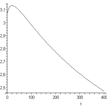
Figure 6: Consumption decrease along the LA curve t∈(0,400)

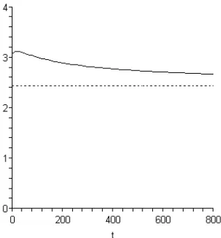
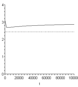
Figure 8: Consumption along the TCC or LD curve

recalculatec(d) andb(d)using our main criterion - constant consumption over time in the long

run (asymptotically constant consumption) instead of the least negative output shock during

transition period. In other words we should solve a system of equations: L(d,α,β) = 1 plus

equations for b(d) and c(d) ((11) and (13)). An example with α = 0.3 andβ = 0.05 gives us

d = 8.0, c = 0.01022, b = ₋0.023196. In this case the maximum negative output shock takes

place a little bit earlier (tmax = 20.1) in comparison with tmax = 22.82 for the LA curve; the

value of the shock is larger (Amax =−0.0767) in comparison withAmaxLA =−0.07605,but the

shock is weaker than for the curve (3), for which Amax=−0.08466.

To check that the level of consumption along this curve, which we can call the “Transition

Constant Consumption” (TCC) curve, is far enough from zero, we can solve numerically

dif-ferential equation fork(t)10 _{and then plotc(t)(Fig. 8). The value of constant consumption for}

thet, big enough, is around cconst = 2.42801.

The maximum value along the TCC curve is cmax = 3.126 at t = 16.6. As we can see,

cconst < c0 = 3.078,11 but rather far from zero. Since we have bounded decrease of consumption

along this curve, we can call it also the “Limited Decline” (LD) curve.

6

Consumption

Growth,

Transition

Curves,

and Generalized Rawlsian Criterion

Another interesting case is the behavior of infinitely growing consumption whenL(d,α,β)<1.

What is the “cost” of this growth? And can it be “optimal” in some sense or is it just a result

of overinvestment? An example with L(7.5671,0.3,0.05) = 0.9 gives us the long-run growing

consumption (Fig. 9) with the same c0, but cmax = 3.1248 at t = 16.2 and cmin = 2.6817 at

tmin = 3035. Consumption exceeds c0 aftert = 1.144·106. The dash line is the asymptote for

the LD curve (Fig. 8).

Negative effects or the “cost” of the long-run consumption growth along this curve,

com-pared with the TCC or LD curve are:

1) cmax is a little bit less, than for the LD curve (3.1248 vs. 3.126);

2) peak of negative shock on output is a little bit stronger (-0.0769 vs. -0.0767) and takes

place on 6 months earlier (t= 19.65vs. t= 20.1).

The example is an illustration of the answer to the question “what is worse”: a small

decrease of consumption in the present or the depriving of oneself and (or) one’s descendants of

any prospects for improving their lives in the future. According to Rawls’s maximin principle, it

is obviously a pattern of overinvestment. But actually Rawls objected to applying his maximin

principle (or as he call it “difference principle”) to the questions of justice among generations

11_{G.B. Asheim [2] considers a theoretical example where the consumption decreases to a sustainable level}

Figure 9: Long-run consumption growth for L(d,α,β) = 0.9

because of unacceptable consequences: “The principle is inapplicable and it would seem to

imply,... that there be no saving at all”([38], p.291). As a solution of the problem Rawls suggests

that the difference principle must be restricted by the additional, “just savings principle”([38],

p.285). But Rawls challenges the possibility of its construction in a precise form: “I believe

that it is not possible... to define precise limits on what the rate of savings should be. How

the burden of capital accumulation and of raising the standard of civilization and culture is to

be shared between generations seems to admit of no definite answer” ([38], p. 286). And there

is a question: why such a plausible and attractive principle for intragenerational questions can

not be extended to problems of intergenerational justice? And why we can not deduce the just

savings principle from the main principle? Where is the essential source of this contradiction?

According to Rawls it is very important to define precisely relevant positions of persons (or

generations) for which we will test different theories of justice: “...selection of relevant positions

person holds two relevant positions: that of equal citizenship and that defined by his place in

the distribution of income and wealth”([38], p. 96). Income and wealth (exchangeable goods)

are used by Rawls as indicators of relevant position in his successive works also (e.g., [39], p. 58,

[40], p.76, p. 181). A.K. Sen [42] has suggested adding some not exchangeable goods such as

measures of development of personal capacities, and, as T. Scanlon has offered, “the avoidance

of chronic physical pain” ([41], p. 41). But there are a number of contributions supporting

the idea that for estimating utility and, consequently, relevant position, it is not enough to

calculate some vector of measurable static indicators. “We can ask,... how well a person’s life

is going and whether that person is...better offthan he or she was a year ago” ( [41], p. 18).

And there is evidence that has “...documented the claim that people are relatively insensitive

to steady states, but highly sensitive to changes...” and “...the main carriers of value are gains

and losses rather than overall wealth” ([20], p. 148). We just can consider, e.g., two persons

with identically the same level of consumption and other not exchangeable goods but the first

one was a billionaire, who lost her fortune just yesterday and the second was a poor peasant,

who improved her live due to a good luck or (and) diligence and a good education. Each will

surely evaluate the quality of her life currently differently. And having no information about

her position in society (“behind a veil of ignorance” [38], pp. 136-142), it looks quite plausible

that any person will choose a theory according to which she will count on a maximum support

from society in a most desperate situation and this “reflex” does not necessarily imply that she

would base her “claim” on the worst static indicators in the current period.

An important element in Rawls’s approach to defining the least advantageous person is

that actually she is not a single person but rather a representative of the “least fortunate

(time-component of the theory) we should consider the least advantageous generation as

rep-resented by a person who stands for the group in the “least fortunate period”. This means

that the person must live during some finite period of time and she doesn’t know how long

this period is. Alternatively if we consider this person as a model of all generations then we

can assume that she lives infinitely. In either case it must be the same person; in the same

way as when we compare utilities of contemporaries, we pick up them from the same time

period. When we consider the dimension “people” we don’t consider the dimension “time” and

vise versa. And since estimation of a person’s utility depends on her “progress”, and only her

“prehistory part” of this progress is available to affect this estimation, the question of savings

can be solved within this period without considering representatives of other generations. We

want to stress that the question of just savings can (not must) be solved within one generation

and this means that we can introduce overlapping generations as an added complication in

order to examine additional effects. Indeed there are persons who have no children but they

do savings to buy a car or a house, there are families who have children but they frankly think

that it will be much better for their children to be self-supporting, and nevertheless they also

do savings to improve their own progress or prevent decline. And we can not say that these

examples exhibit irrational behavior.

Hence, evaluation of one’s life quality should include not only calculations of some static

indicators, but rather such indicators combined with time-changes of variables (growth or

re-cession) or differences in consumption from previous years. Assume, for simplicity, that utility

from consumption has the formu(c) =c. For discrete time and taking into account the

evalua-tion of some prehistory, the generalized Rawlsian criterion maximizes the minimal over all time

wheren+1is a length of a “memory interval” (each person lives at leastn+1periods), the sum

n

i=0wi(ct−i−ct−i−1) is thought of as the person’s memory of earlier utility levels or the

“his-torical benchmark level” ([4] , p. 1257) and distribution ofwi over time ( wi = 1, wi ∈[0,1])

depends on individual adjustment to changes in consumption. This form of individual welfare

is close to K.J. Arrow [1], P. Dasgupta [6], J. Lane and T. Mitra [25], and N.V. Long [28]. The

two differences are: 1) we take into account not the consumption of descendants (ct+1) but the

past consumption of the same person; 2) we evaluate past consumption not in absolute value

but as a component in the process of comparing the past with our present condition (gains and

losses). We want now to show that even for such an “egoistic” model, the generalized Rawlsian

principle can imply intertemporal consumption growth. Taking into account “past experience”

in its simplest form and making use of continuous time and following Rawls strictly12_{, the}

corol-lary of the Generalized Rawlsian Criterion for intertemporal distribution (c(t) is continuously

differentiable) can be written, e.g.13, as:

wc(t) + (1₋w)c(t) =˙ γ =const for any t, w_∈[0,1], (17)

It means (forc >˙ 0) that a person in the future with higher consumption and less growth must

“feel the same emotional evaluation” or have the same utility level of her “position” as she

feels in the present with less consumption and higher value of c(t).˙ Note that for γ < c0w we

have a case of generalized “fair Rawlsian decline”;14 a person in the present has not only higher

12_{We assume, according to Rawls, the fulfillment of hisfirst principle (“Each person is to have an equal right}

to the most extensive total system of equal basic liberties compatible with a similar system of liberty for all”) and we will apply the second principle in absolutely the same way (“Social and economic inequalities are to be arranged so that they are...to the greatest benefit of the least advantaged...” [38], p. 302), but maximize the minimal value of some combinationc(t)withc˙(t).

13_{The author introduced an example of utility in form (17) independently of N.V.Long ([28], p.17) andc˙here}

has a different meaning. It is an estimation of person’s “prehistory” which influences her evaluation of current consumption, rather then expected future consumption as it is in N.V. Long’s interpretation.

14_{We have no proof that present economic growth is not a pattern of overshooting and so we must define not}

level of consumption but also higher rate of decline, than she has in the future, so that the

weighting according to (17) yields the same utility for each period. In the long run it reminds

the consumption behavior along the LD curve after the point of maximum (Fig. 8).

Expressing c(t)from (17) with c0 =c(0) we have

c(t) = 1

w γ−e

− w

1−wt(γ−c

0w) (18)

with

˙

c(t) = 1 1−we

− w

1−wt(γ−c

0w),

and then the path of net investment N(t)is a corollary of the Rawlsian “difference principle”.

For utility in form (17) N(t) was obtained by N.V. Long [28]:

N(t) =c(t)g(t),˙

where

g(t) =

∞

t

e− tτ[ w

1−w+fK(s)ds]dτ >0.

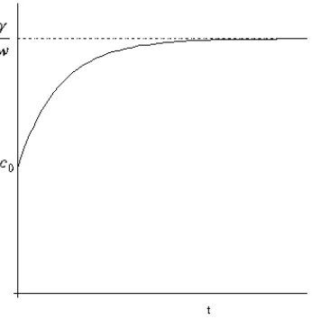
Observe that limt_→∞c(t) = 0˙ or we have a case of limited growth (Fig. 10) for γ > c0w

(even without overlapping generations as in [35] and without discounting of maximin as in [21])

and this curve isdesirable in a sense “...that an extra bit of consumption at t is more valuable

than the sameextra bit att+ 1, since individuals will, in any case, have more consumption at

t+ 1.” ([7] p. 284) But observe also that we have limited decline forγ < c0w, and identically

constant consumption (as in the Hartwick rule) forγ =c0w.

So, for the LD curve we have the consumption behavior, which in the long run is “close”

Figure 10: Generalized “fair Rawlsian growth” (18), w= 0.5

“cost” of the impossibility of an instantaneous switch to the Hartwick curve is an infinite but

limited decline of consumption to the value which is less than c0. In the sense of (17) this is

the path which is “close” to optimal, except for the rate of its decline15_{. The value of w is}

supposed to be defined by the government. We do not claim that everybody favors this type

of just path, particularly when it is apparent that rather small sacrifices in present can bring

slow but unlimited growth in the long run (Fig. 9).

For those, who prefer this form of intertemporal distribution, the more appropriate

consump-tion utility funcconsump-tion would be the funcconsump-tion with essential factors and the constant elasticities

of marginal utility, e.g., the Cobb-Douglas case. Then the rule of intertemporal distribution is

cwc˙1−w =γ =const, (19)

which forw= 1 is also the corollary of the regular Rawlsian principle. Integration of (19) gives

us

c(t) =c0(1 +μt)ϕ (20)

where

c0 =c(0),μ=

1 1−w

γ

co

1 1−w

,ϕ= 1₋w

or a pattern of unlimited (quasi-arithmetic, [3], p. 5) growth which (forwclose to 1) looks like

the part of the curve on Fig. 9 after the point of minimum.

Utility can be written more generally as a CES function, or as a function with a variable

elasticity where the elasticity of factor substitution andware to be chosen by the government.16

Then the specific just savings principle can be deduced for the specific utility function and the

extraction path (transition curve) can be adjusted to approach as close as possible (depending on

constraints) the asymptotically optimal (in the long run) pattern of intertemporal distribution

of consumption.

Rawls holds the asymmetry of intergenerational relations to be the reason for being unable

to apply his maximin principle: “It is now clear why the difference principle does not apply

to the savings problem. There is no way for later generations to improve the situation of the

least fortunate first generation. The principle is inapplicable and it would seem to imply, if

anything, that there be no saving at all. Thus, the problem of saving must be treated in

another fashion” ([38], p. 291). Indeed intergenerational asymmetry influences the process of

just intergenerational allocation. That is why Rawlsian just distribution among contemporaries

allows inequality in utility unlike intergenerational allocation which implies the same utility (for

16_{And in turn, our moral evaluation of government activity in maintaining some rate of economic growth}

the combination of consumption and “progress”) for the same person but generally not the same

level of consumption and not a zero net saving rate. So using this approach for a definition of a

person’s relevant position we “reduce” the problem of just savings to the problem of the choice

of a proper form of the utility function.

The choice of utility function involves another important problem, namely the problem of

dynamic inconsistency. This means that for an infinitely lived person we do have a rather

“good” function like (18) or (20). But if we reformulate the problem as a set of problems

each of which is solved by a member of the overlapping or subsequent generations, we

(de-pending on concrete form of utility function) can obtain a path which is continuous, but has

points of discontinuous derivatives at the moments of time where another generation chooses

its own optimal path using the same approach. And the resulting combination of these paths

will generally not coincide with the path of an infinitely lived person. Or if we assume that

an infinitely lived person will check and recalculate her path at each moment of time then we

will observe that she always changes her preferences and this seems to contradict the usual

assumptions of rational behavior. Therefore, for models with always rational agents we must

pick a form of the utility function which 1) induces dynamically consistent paths (constraint);

2) in the best way reflects real agents’ preferences (criterion). But then our agenda becomes

extremely complicated. From our perspective dynamic inconsistency needs a separate

consid-eration.17 _{Moreover since preferences can often change over time even for rational agents [8]}

and in addition we have uncertainties with initial conditions (e.g., estimation of initial stock

S0), the optimal path of extraction will generally need a correction and an adjustment of the

17_{One of thefirst works on dynamic inconsistency was a paper of R. Strotz [46], for non-renewable resources}

parameters of the transition curve from time to time. And then the resulting path apparently

will not be a “globally optimal” curve but rather will “...be compared to the course of a dog

running across a field toward his master, while the master walks along the road”[27].

7

Concluding Remarks

It deems natural for the government, committed to switching to sustainable path, to consider

the problem of minimizing the short-run negative consequences of moving to such a path. We

observe that the so-called optimal short-run transition path involves an interval of zero

con-sumption and this runs counter to the government’s primary goal of pursuing intergenerational

justice principle in the long run.

Consideration of the long-run consumption behavior along possible transition curves shows

that even for inefficient curves there is a path of extraction with asymptotically constant

(sep-arated from zero) consumption over time. The short-run negative shock along this transition

path is small for our numerical example based on observed world oil extraction data. Moreover,

a “worsening ” of the short-run situation (shortening the period of transition and introducing

a stronger negative shock on output) yields the possibility of slow, but unlimited growth of

consumption in the long run. In other words the transition curve (to be exact, the single free

parameter -d) can be fitted to satisfy desirable qualitative behavior of consumption in accord

with the various optimality criteria in the long run. And it again raises the long-standing

ques-tion about the fairest ethical theory for the distribuques-tion of consumpques-tion across generaques-tions. If

decreasing the rate of oil extraction is really necessary, which criterion we must follow? 18

Aside from equivocation on our main welfare criterion there are some other questions and

limitations of the model we have presented.

(1) We examined transition curve as interior solution neglecting restrictions imposed by

technical possibilities and difficulties connected with the saving rate changing. Constraints

on the speed of changing savings behavior can restrict us from implementing even the path

of extraction with asymptotically constant consumption not speaking of paths with unlimited

growth in the long run (questions of optimal path existence and uniqueness).

(2) There is an interesting question of the optimal program stability with respect to initial

conditions.

(3) There is one more interesting question of the comparative estimation of the consumption

behavior, considered in this paper with the consumption behavior along the efficient transition

paths.

(4) Transition curve can be constructed in different class of functions, e.g., as a solution of

calculus of variation problem.

We also assumed that:

(5) Cost of extraction is zero and population is constant though it would be interesting to

consider the problem of transition when these values are variables.

(6) There is no time lag between the moment of oil extraction and correspondent increment

of man-made capital which is not true if we invest oil rent in the development of alternative

technologies.

(7) All oil rent is invested into reproducible capital. In general, this is not observed and we

should consider some period of increasing investments along some smooth (maybe

hysteresis-like) curves and examine the influence of this curve on long-run consumption behavior.

position though there is evidence that “Losses loom larger than gains...” ([20], p. 148).

We think that all these questions need special careful consideration in separate papers.

References

[1] Arrow K.J. (1973), Rawls’ Principle of Just Saving // Swedish Journal of Economics. Vol.

75, No 4.

[2] Asheim G.B. (1994), Net National Product as an Indicator of Sustainability // The

Scan-dinavian Journal of Economics. Vol. 96, No 2.

[3] Asheim G.B., Buchholz W., Hartwick J.M., Mitra T., Withagen C. (2005), Constant

Sav-ings Rates and Quasi-Arithmetic Population Growth under Exhaustible Resource

Con-straints. CESifo Working Paper No 1573, October 2005.

[4] Barberis N., Huang M. (2001), Mental Accounting, Loss Aversion, and Individual Stock

Returns // Journal of Finance. Vol. 56, No. 4.

[5] Castanheira M., Roland G. (2000), The Optimal Speed of Transition: A General

Equilib-rium Analysis // International Economic Review. Vol. 41, No 1.

[6] Dasgupta P. (1974), On Some Alternative Criteria for Justice Between Generations //

Journal of Public Economics. Vol. 3, No 4.

[7] Dasgupta P., Heal G. (1979), Economic Theory and Exhaustible Resources. Digswell Place:

Cambridge University Press.

[8] Dasgupta P., Maskin E. (2005), Uncertainty and Hyperbolic Discounting // American

[9] Duesenberry J. (1949), Income, Saving and Theory of Consumer Behavior. Cambridge

MA: Harvard University Press.

[10] Farmer K., Wender R. (2003), A Two-Sector Overlapping Generations Model with

Het-erogeneous Capital // Economic Theory. Vol. 22, No 4.

[11] Fisher C., Withagen C., Toman M. (2004), Optimal Investment in Clean Production

Ca-pacity // Environmental and Resource Economics. Vol. 28, No 3.

[12] Fuss M. A. The Demand for Energy in Canadian Manufacturing // Journal of

Economet-rics. Vol. 5, No 1.

[13] Gray L.C. (1914), Rent Under the Assumption of Exhaustibility // Quarterly Journal of

Economics. Vol. 28, No 3.

[14] Griffin J.M., Gregory P.R. (1976), // The American Economic Review. Vol. 66, No 5.

[15] Grout P. (1977), A Rawlsian Intertemporal Consumption Rule // The Review of Economic

Studies. Vol. 44, No 2.

[16] Halvorsen R., Ford J. (1979), Substitution among Energy, Capital and Labor Inputs in

American Manufacturing. In: Advances in the Economics of Energy and Resources. Vol.

1. Ed.: R. Pindyck. Greenwich, Conn.: JAI Press.

[17] Hartwick J.M. (1977), Intergenerational Equity and the Investing of Rents from

Ex-haustible Resources // The American Economic Review. Vol. 67, No 5.

[19] Hotelling H. (1931), The Economics of Exhaustible Resources // The Journal of Political

Economy. Vol. 39, No 2.

[20] Kahneman D., Varey C. (1991), Notes on the Psychology of Utility. In: Interpersonal

Com-parisons of Well-Being. Eds.: J. Elster and M.S. McPherson. NY: Cambridge University

Press.

[21] Kaganovich M. (2000), Decentralization of Intertemporal Economies with Discounted

Max-imin Criterion // International Economic Review. Vol. 41, No 4.

[22] Kimia B.B., Frankel I., Popescu A.M. (2003), Euler Spiral for Shape Completion //

Inter-national Journal of Computer Vision. Vol. 54, No 1-3.

[23] Konow J. (2003), Which Is the Fairest One of All? A Positive Analysis of Justice Theories

// Journal of Economic Literature. Vol. 41, No 4.

[24] Kuznets S. (1946), National Product Since 1869. New York: National Bureau of Economic

Research.

[25] Lane J., Mitra T. (1981), On Nash Equilibrium Programs of Capital Accumulation under

Altruistic Preferences // International Economic Review. Vol. 22, No 2.

[26] Leininger W. (1985), Rawls’ Maximin Criterion and Time-Consistency: Further Results

// The Review of Economic Studies. Vol. 52, No 3.

[27] Leontief W. (1959), Time-Preference and Economic Growth: Reply // The American

Economic Review. Vol.49, No 5.

[29] Long N.V. (2006), A Mixed Bentham-Rawls Criterion for Intergenerational Equity.

Man-uscript. McGill University.

[30] Magnus J.R. (1979), Substitution between Energy and Non-Energy Inputs in the

Nether-lands 1950-1976 // International Economic Review. Vol. 20, No 2.

[31] Nemoto K. (2005), High Oil Prices Dampening Asia-Pacific Product Demand // Oil &

Gas Journal. Vol. 103, No 46.

[32] Newbery D.M.G. (1981), Oil Prices, Cartels, and the Problem of Dynamic Inconsistency

// The Economic Journal. Vol. 91, No 363.

[33] Nordhaus W.D., Tobin J. (1972), Is Economic Growth Obsolete? In: Economic Growth,

5th Anniversary Colloquium, V, National Bureau of Economic Research, New York.

[34] Nordhaus W.D. (1993), Rolling the ’DICE’: An Optimal Transition Path for Controlling

Greenhouse Gases // Resource and Energy Economics. Vol. 15, No 1.

[35] Phelps E.S., Riley J.G. (1978), Rawlsian Growth: Dynamic Programming of Capital and

Wealth for Intergeneration “Maximin” Justice // The Review of Economic Studies. Vol.

45, No 1.

[36] Pindyck R.S. (1979), Interfuel Substitution and the Demand for Energy: An International

Comparison // Review of Economics and Statistics. Vol. 61, No 2.

[37] Poterba J. (1988), Are Consumers Forward Looking? Evidence from Fiscal Experiments

[38] Rawls J. (1971), A Theory of Justice. Cambridge: Belknap Press of Harvard University

Press.

[39] Rawls J. (2001), Justice as Fairness. Cambridge: Belknap Press of Harvard University

Press.

[40] Rawls J. (2005), Political Liberalism. NY: Columbia University Press.

[41] Scanlon T.M. (1991), The Moral Basis of Interpersonal Comparisons. In: Interpersonal

Comparisons of Well-Being. Eds.: J. Elster and M.S. McPherson. Cambridge: Cambridge

University Press.

[42] Sen A.K. (1982), Equality of What? In: Choice, Wefare and Measurement. Cambridge

MA: MIT Press, pp. 353-372.

[43] Solow R.M. (1974), Intergenerational Equity and Exhaustible Resources // The Review

of Economic Studies. Vol. 41. Symposium on the Economics of Exhaustible Resources.

[44] Stiglitz J.E. (1974), Growth with exhaustible natural resources: efficient and optimal

growth paths // The Review of Economic Studies. Vol. 41. Symposium on the Economics

of Exhaustible Resources.

[45] Stollery K.R. (1991), Capital-Resource Substitution and the Discount Effect in Depletable

Resources // Southern Economic Journal. Vol. 58. No 2.

[46] Strotz R.H. (1955), Myopia and inconsistency in dynamic utility maximization // Review

8

Appendix (proof of the Proposition 2)

For the economy with a Cobb-Douglas production function q = kα_rβ _{and investment covered}

by resource rent in k˙ =βq, expression [·] in the right hand side of (15) is

˙

k q −

(1₋β)

α

k q

˙

r

r =β−(1−β) k

αq

˙

r r.

In the long run r <˙ 0and(1₋β), k,α, q, r > 0. Then we can rewrite the last equation as

[·] =β+ (1₋β) k

αq

|r˙|

r ,

which means that [·] = 1 if and only if k

αq |r˙|

r = 1,and generally

sgn{1−[·]}= sgn 1− k

αq

|r˙|

r .

So, in order to examine the behavior ofq(t)andc(t),we can compare k

αq |˙r|

r or 1

αk1−αr−(1+β)|r˙|

to unity where k(t) is an unknown function. An attempt to find k(t) from the differential

equationk˙ =βkα_rβ _{gives us k}1−α _{=β(1−α)I(t), where}

I(t) = r(t)βdt=r0β

(1 +ρt)β

(1 +ct)β(d−1)dt=r

β

0I1(t),

and ρ = c(d₋1) +A0/r0. The integral I1(t) can be expressed in elementary functions using

Chebyshev substitutions if we setd= 12 and β = 0.1,0.2,0.3, and so on. Thus, for β = 0.2

k1_0.2−α(t) =β(1−α)r

β

0a1c−10β

ρ(p+ 1) (ac+bc)

(p+1)

− ac

1 +ρt+bc

(p+1) _+k1−α

0 , (21)

whereac= 1− _ρc, bc= _ρc, p=β(1−d). And forβ = 0.3

k_0.31−α(t) = β(1−α)r

β

0a1c−10β

× (ac+bc)(p+1)[ac(p+ 1)−bc]−

ac

1+ρt+bc

(p+1) ac(p+ 1)

1 +ρt −bc +k

1−α

0 .

k0 must be the same for any curve, and so it can be evaluated for our economy using equation

(1) for the Hartwick curve in terms of output q0 =q(0) :

k0 =−

αq0r0

A0H

,

where q0 can be set equal to unity and A0H = r˙Hart < 0 for the Hartwick curve. We can

use (21) and (22) for a detailed analysis of capital (e.g., asymptote for t _{→ ∞}), output, and

consumption along some transition curve. We must restrict attention to the cases β = 0.2 or

β = 0.3. The expression for k(t), given β = 0.1 is lengthier than (21) or (22) and we will not

consider it here. We are interested in cases with β < 0.1 in which according to Chebyshev

theoremk(t) can be expressed in elementary functions for relatively large values of d.19

However we can consider the asymptotic behavior of expression k1−α_r−(1+β)_|

˙

r|. Note, that

limt→∞k1−α(t) =∞,sincek˙ =βq >0for anyt≥0.And the asymptotic behavior ofr−(1+β)|r˙|

is

lim

t→∞r

−(1+β)_|

˙

r| = lim

t→∞

(1 +ct)d−1

r0(1 +ρt) 1+β

A0+bt

(1 +ct)d

= 1 r0

1+β

lim

t→∞

(1 +ct)(d−1)(1+β)

(1 +ct)d ·

|A0+bt|

(1 +ρt)1+β (23)

= 1 r0

1+β

lim

t→∞

1 +ct 1 +ρt

β

· |A0+bt|

1 +ρt ·(1 +ct)

β(d−2)−1

= 1 r0 1+β · c ρ β

· |b|

ρ ·tlim→∞(1 +ct)

β(d−2)−1

19_{An integral τ}β_(a

c+bcτn)pdτ, where τ = 1 +ρt,can be expressed in elementary functions only in cases

1)p- integer; 2) β+1

n - integer; 3)

β+1

n +p- integer. In our casep=β(1−d)and forβ∈(0,1) andn= 1we

can use the third case. Then we have a condition: β(2₋d) + 1 =N must be an integer. From thefiniteness of the resource we have constraint d >3or N <1₋β and so, the minimum feasible (N = 0) value of dfor

or

lim

t→∞r

−(1+β)_|

˙

r|=

⎧ ⎪ ⎨ ⎪ ⎩

0, β(d₋2)<1,

1 r0 1+β c ρ β

|b|

ρ, β(d−2) = 1,

∞, β(d−2)>1.

This means that forβ(d₋2)_≥1we have our output and consumption asymptotically

decreas-ing:

lim

t_→∞sgn{1−

1

αk

1−α_r−(1+β)_|

˙

r|}= lim

t_→∞sgnq˙=−1

or the first expression in statement (16) of the proposition. The most interesting case is when

β(d−2)<1.Then using (23) we have

lim

t→∞k

1−α_r−(1+β)_|

˙

r|=_∞·0 = lim

t→∞

k1−α

1/(r−(1+β)_|r˙|) =

∞ ∞

= lim

t→∞

d[k1−α_]/dt

d[1/(r−(1+β)_|r˙|)]/dt

= 1 r0 1+β c ρ β

|b|

ρ tlim→∞ (1−α)k

−α_k/˙ d (1 +ct)−β(d−2)+1

dt = 1 r0 1+β c ρ β

|b|

ρ

1₋α

c[1₋β(d₋2)]tlim→∞

βrβ

(1 +ct)−β(d−2)

= 1 r0 1+β c ρ β

|b|

ρ

(1−α)βr₀β c[1₋β(d₋2)]tlim_→∞

(1 +ρt)β

(1 +ct)β(d−1) ·(1 +ct)

β(d−2)

= 1 r0 1+β c ρ β

|b|(1₋α)βrβ₀

ρc[1−β(d−2)]tlim→∞

1 +ρt 1 +ct

β

.

Andfinally we have

lim

t_→∞k

1−α_r−(1+β)_|

˙

r|= |b|(1−α)β r0ρc[1−β(d−2)]

,

where b=b(c(d), d) (see (11)) andc=c(d) (see (13)). Thus forβ(d−2)<1

lim

t→∞sgnq˙= limt→∞sgn 1−

1

αk

1−α_r−(1+β)_|

˙

r| = 1₋ |b|(1−α)β r0αρc[1−β(d−2)]

,