Tuning of the Pressure Equation in the Natural Gas Transmission Network

Tuning of the Pressure Equation in the Natural Gas

Transmission Network

Naser .HajiAliAkbari

The Petroleum University of Technology (Iran) Iran, Ahwaz, The Petroleum University of

Technology

R. Mosaiebi Behbahani

The Petroleum University of Technology (Iran) Iran, Ahwaz, The Petroleum University of

Technology

ABSTRACT

The best and most economical way of transportation of natural gas in immense scale and for a long time is pipeline. In this paper a small portion of the natural gas transmission networks in Iran has been analyzed, Part of the main export pipeline with some branch to Local consumers.

From the perspective of a manager or engineer of Gas industry, Gas distribution network is a set of parameters; the most important parameter is pressure at any point of gas network. Engineering Software estimates the pressures based on the pressure equation; these equations have always some errors, sometimes the error is a too much as far as could be cause serious problems in gas distribution. In general gas equation is Connection between flow pressure pipelines; based on temperature, roughness, compressibility factor, density gas pipeline specifications and environmental changes. In this research we have tried to adapt the amount of pressure based on Roughness values changes.

Recently, several statistical techniques are used to solve such problems, in this study, the genetic algorithm is used. Along with error correction it has time saving compared to the analytical methods.

Tuning process in this network System error can be reduced by up to 8 times in first step and it can be insignificant if the strong computer Processor or sufficient time be available.

General Terms

P - pressure Q - actual flow rate T - temperature

Z - gas compressibility factor

Keywords

Gas transmission, Pipeline, Optimization, Pressure equation, NG behavior simulation, Statistical calculations, Tuning

1.

INTRODUCTION

Gas, as a result of the storage difficulties, needs to be transported immediately to its destination after production from a reservoir. There are a number of options for transporting natural gas energy from oil and gas fields to market (Rojey et al., 1997; Thomas and Dawe, 2003). These include pipelines, liquefied natural gas (LNG), compressed natural gas (CNG), gas to solids (GTS), i.e., hydrates, gas to power (GTP), i.e., electricity, and gas to liquids (GTL), with a wide range of possible products, including clean fuels, plastic precursors, or methanol and gas to commodity (GTC), such as aluminum, glass, cement, or iron [4].

Gas Network Management

Gas network management Means: setting the pressure and input Equipment’s power; so that doesn’t accrue any pressure drop or abnormal pressure in the network. The manager tool for this purpose is dispatching, Dispatching is a set of tools and software which Connect between the equipment and engineers. Equipment generally has little specified error value that will be negligible by calibration; but softwares are more challenging, this will be discussed in following.

General Flow Equation

Based on the assumptions that there is no elevation change in the pipeline and that the condition of flow is isothermal, the integrated Bernoulli’s equation is expressed by Equation (11-1) (Uhl, 1965, Schroeder, 200(11-1)[4]:

Where Qsc is standard gas flow rate, measured at base

temperature and pressure, ft3_/day;

Pipelines are usually not horizontal; however, as long as the slope is not too great, a correction for the static head of fluid (Hc) may be incorporated into Equation (11-1) as follows

(Schroeder, 2001) [4].

Error definition

Based on the review Of Data taken from network measurement system Significant amount of error is has been observed.

Error in performed analysis means:

The difference between the pressure data that has been read from the pressure control station (And outbound of the network) and the predicted quantities from the equations used in the software.

E= Pout(measurement) – Pout(P,D,z,L,T,μ,…)

This value has been reduced during the history by provided newer Equations.

Sources of Error

The answer is pipelines condition and what will happen in feature is ambiguous. Such as:

1 - Aging the pipes; this factor is influenced by many parameters (such as temperature tubes per minute, precise amounts of alloy composition, metallurgy metal tube sex, gas ...)

2 – Environment; Temperature and weather forecast for the next few days Is an approximate so Temperature and weather exact forecasting for over than 30 years is impossible

The only way in this issue is using statistical optimization for fixing the Equations which used in softwares.

Such corrections are common in developed countries, for example (in 2012), ATMOS International Limited has carried out extensive research on the Subsea Pipeline Models [3]. Which leads to: Better estimates of the hydraulic capacity and the Estimated Time of Arrival will be achieved by tuning the effective roughness and the heat transfer of the pipeline models.

We ask that authors follow some simple guidelines. In essence, we ask you to make your paper look exactly like this document. The easiest way to do this is simply to download the template, and replace the content with your own material.

2.

NETWORK

SIMULATION

Studied Network in The paper is a branched network (Figure 4) Simulation codes have written Based on the traditional equations (in this study AGA are chosen)

In this study the temperature changes are ignored, the reason for this is: a) pipelines are buried b) Attempts to correct the equation only Based on the roughness is modification

Most common Equations

In order to construct a pipeline from a conventional equation for gas transmission network this is used in most National Iranian Gas Company’s software:

AGA

The AGA fully turbulent is the most frequently recommended and widely used equation L high-pressure, high-flow-rate systems for medium- to large-diameter pipelines. It predicts both flow and pressure drop with a high degree of accuracy, especially if the effective roughness values used in the equation have been measured accurately [1].

The AGA folly turbulent equation has the following form in Imperial Units.

Where:

Qb = gas flow rate at base conditions, SCF/D

Tb = temperature at base condition, 520 °R

Pb = pressure at base condition, 14.7 psia

Where the transmission factor is defined using the Nikuradse equation [1]:

Optimization

The most important part optimization is determining objective function, the Strategies for Process and finding disputed part of the equations (This is usually one of the pipelines specifications).

First the pipeline equation is considered:

Almost every one of the parameters in the equation can be taken into account as an objective function but there are some issues that should be considered and no one can decide without thorough review of the pipeline and Mastering in instruments on pipelines. Flow (Q) and pressure (P) are connected and both can be the objective, p has some Advantages (1. It can be measured easily 2.it can be measured exact 3. Pressure has very common units and in most time it is psi)

Eventually there is no Fundamental difference but pressure has some advantages so pressure was considered as the objective function.

The equation can be rewriting as below:

Rewritten in terms of the pressure is not necessary, but it is better understanding of dependencies and Sensitivity analysis.

After passage of time will be two sets of data: 1 - Series pressures calculated in software

2 - Series of reports of pressure measurement systems

Genetic Algorithm

The genetic algorithm is a method for solving both constrained and unconstrained optimization problems that is based on natural selection, the process that drives biological evolution. The genetic algorithm repeatedly modifies a population of individual solutions. At each step, the genetic algorithm selects individuals at random from the current population to be parents and uses them to produce the children for the next generation. Over successive generations, the population "evolves" toward an optimal solution [2].

At each step, the genetic algorithm uses the current population to create the children that make up the next generation.

GA in MATLAB

One of the most practical software for academic Semi-industrial research in chemical engineering is MATLAB. In this study codes was written in MATLAB based on AGA equation.

For optimization of the problem ‘Optimization Toolbox (Optimtool)’was used.

between 10to 10000 micro inch, fitness scaling was rank, migration was forward, and no hybrid function and the crossover was Heuristic (returns a child that lies on the line containing the two parents).

Heuristic crossover [2]:

Child = parent2 + R * (parent1 - parent2)

In the optimization fitness function was Ke (roughness value), the number of variables was n umber of pipes and the objective function was sum of squared differences (Σ(Pi

2

-P’i2)).

3.

RESULT

The case was a real sample of gas transmission pipelines in Iran. It’s the Part of a major pipeline that has branches in several small towns.

This analysis has been based on AGA and Colebrook-White equation. In this paper, the error is:

E= Pout(AGA) or Pout(Colebrook-White) - Pout(measurement)

Programming is done in the objective function (which should be minimized):

O.F= Σǀ[Pi 2

(measurement) - Pi

2_{(Calculation)]ǀ}

Accurate modeling was performed assuming isothermal network model based on roughness values, default values are provided in table 1.

As can be seen in Table in 6 points in a network is the destination of the parameters, there are some significant errors. These errors are related to the timing and conditions provided there is no pressure equation and Claimed to have provided with no errors equation.

But this is not an insoluble problem. One of the best solutions is uses of optimization process; this means that pressure equations of pipelines to be corrected periodically so that in the next period they will predict the best possible answer. Only a very limited number of studies based on genetic algorithm optimization process can give satisfactory results (table 2).

Although these results may not be perfect, but the error reduction about 20% by only spend a few minutes, is acceptable. Optimization success rate in this case is a bit difficult, it does not mean it is better or not (definitely is improved), but the success rate is discussed. The reason for this lack is measurable indicators for each section of the pipeline.

Of course, in this part of the network, Optimization criterion is Pressure-tail, in small cities entrance.

By examining the results of the network optimization in limited points limited, for all points results obtained. If the results of these points were not in the objective function no is evaluated (table 3).

As there is a huge difference between the endpoint was not reached until after there is a change.

In The text the Point to zero (without change) are presented as the ultimate optimization.

Total 1. error in steps of optimization (GA)

Mode default Preliminary slight

Total error 125.69 103.9904 85.42134

medium Final Ultimate

48.75652 16.22369 -0.02324

Reaching to the Ultimate point takes tenfold time more than reaching to final point from an economic perspective10 times more for the upgrade successful factor from 87% to 100% is often not justified (justified if there is plenty of time).

Figure 1: Total absolute error

If the kinds of errors are Contemplate, Can be found that there is generally a positive error, which means the default used roughness Increased over time. This is more evident in the main pipeline; Due to the large diameter main pipeline is expected to be less effective over time, while there is The effect is not only less ,But sometimes equal to or greater! The reasons that can be noted: Pipes are older or using worse alloy or material in this pipe.

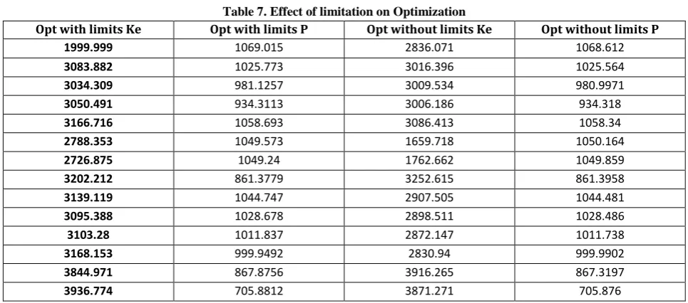
If we change the optimization and remove the previous limits the following answers Will achieved:

If answers of two sets are compared:

Figure 2: The effect of Range restrictions on Optimization

Both answers are good answers of pressure. But by a short review on roughness values can be found the limitations are reasonable.

-50 0 50 100 150

0 10000 20000 30000

Sum (abs(Pcalc-Psetpoint))

Total error

0 1000 2000 3000 4000 5000

1 2 3 4 5 6 7 8 9 10 11 12 13 14 15 16 17

Because the passage of time always increase the pipe’s roughness; roughness should be much greater; its compliance in limited mode.

Now if the results of the optimization period 1 be considered for network optimization in second and other period following differences are observed:

Figure 3: GA with initial value

By insert the Optimized values from period 1 for period 2, (network flows and pressures have changed), rate to achieve response will increase in 1000times.

Time saving

In this study, the genetic algorithms are used to optimize this method is a statistical method that can be used to optimize the most simulated process.

Response rate in this way is much higher, if the number of computations performed in two modes:

1 - Calculate all modes and search

2 - Genetic Algorithm Are Considered:

1)

(Number of pixels)No of points _{= (500)}17 _{= 7.629394*10}45

2)

(Number of pixels)*(generation) = 500*25000 = 12500000

In this case, the optimization process by Central Processing Unit: Intel(R) Core2Due @ 2.8GHz take About 10 hours. By A rule of thumb if the number of computations put measure of the speed, the first method will take about Thousands of years.

Usually in a genetic algorithm Analysis is about one or more controversial variables. In this study, roughness is selected

The reason for this choice is more ambiguous than other variables; for pipeline the variable range is between 500 and 5000; this limit is good estimate for common metal pipes.

4.

CONCLUSIONS

From the perspective of, Gas distribution network management there are two important parameters:

 The quantity of gas transmission networks

 Quality services to gas consumers

Software used in the gas industry uses certain pressure equations. The average of the errors are acceptable, But these errors over time due to environmental influences and aging network increases for satisfying the Two parameters the equations are required which Have high accuracy And don’t lose accuracy over time.

Tuning of these equations based on statistical algorithms significantly increase the accuracy, There will be the exact quantity Also quality of service to consumers’ increases that means pressure drop and Gas lost won’t happen and of course there is no abnormally high pressure in the network.

5.

REFERENCES

[1] Pipeline Design and Construction – A Practical Approach. M. Mohitpour, H. Golshan, A. Murray. [2] Kalyanmoy Deb, "Multi-Objective Optimization using

Evolutionary Algorithms", John Wiley & Sons ISBN 047187339.

[3] G. Hanmer, E. Jackson 2012, Tuning of Subsea Pipeline Models to Optimize Simulation Accuracy PSIG, 18 May 2012.

[4] Handbook of Natural Gas Transmission and Processing gives engineers, Saeid Mokhatab, William A. Poe, James G. Speight

[5] Optimization of Chemical Processes Thomas F. Edgar [6] Hydrocarbon Phase Behavior, Tarek H. Ahmed

[7] Introduction to Chemical Engineering Thermodynamics, J. M. Smith, H. C. Van Ness, M. M. Abbott

[8] http://www.mathworks.com/trademarks

[9] Thomas F. Edgar, David Mautner Himmelblau, Leon S. Lasdon, 2001, Optimization of chemical processes, McGraw-Hill.

[10]Rao S.S., 2009, Engineering Optimization Theory and practice, 4th edition, Wiley, USA.

0 5 10 15

0 1000 2000 3000 4000

Sum (abs(Pcalc-Psetpoint))

0 5000 10000 15000 20000 25000

0 1000 2000 3000 4000

TABLES

Table 2. default value errors

Default Value Exact Value Error

1069.127 1030.482 990.6736

949.197 934.318 14.878

1059.937 1051.636

1051.33 1050.020 1.309

887.1947 861.396 25.798

1046.629 1031.204 1015.033 1003.845 893.691

763.3859 705.879 57.506

997.5334

997.2169 983.954 13.262

996.6532 983.716 12.937

Table 3. preliminary GA errors

Preliminary optimization Exact Value Error

1069.015 1029.528 988.7827

946.3142 934.318 11.996

1059.647 1051.179

1050.87 1050.020 0.849

879.8802 861.396 18.484

1046.247 1030.72 1014.447

1003.14 889.321

753.9875 705.879 48.108

996.7163

996.388 983.954 12.433

995.8338 983.716 12.117

Table 4. Errors in all points

Full optimization Exact Value Error

1070.114 1070 -0.11391

1069.751 1069.65 -0.10123

1069.776 1069.73 -0.04643

1069.81 1069.81 2.42E-05

1061.979 1061.82 -0.15858

1061.935 1061.78 -0.15483

1061.933 1061.63 -0.30262

1057.367 1057.62 0.253078

1046.228 1045.41 -0.81751

1007.935 1007.02 -0.91514

994.7845 994.085 -0.69947

991.4283 990.617 -0.81126

983.1795 983.183 0.003468

986.9607 986.481 -0.47972

987.4716 986.948 -0.52359

985.8225 985.903 0.080533

Table 5: Network point’s Optimization steps

default Preliminary slight medium Final Ultimate

1069.127 1069.015 1069.015 1069.015 1069.015 1069.015

1030.482 1029.528 1028.794 1027.216 1025.773 1025.563

990.6736 988.7827 987.2276 984.1648 981.1257 981.1376

949.197 946.3142 943.9261 939.0506 934.3113 934.3145

1059.937 1059.647 1059.466 1059.086 1058.693 1056.892

1051.636 1051.179 1050.861 1050.199 1049.573 1050.389

1051.33 1050.87 1050.547 1049.877 1049.24 1050.02

887.1947 879.8802 873.9576 862.4927 861.3779 861.3955

1046.629 1046.247 1045.969 1045.415 1044.747 1041.736

1031.204 1030.72 1030.348 1029.622 1028.678 1024.377

1015.033 1014.447 1013.988 1013.067 1011.837 1006.246

1003.845 1003.14 1002.585 1001.453 999.9492 993.0712

893.691 889.321 885.4802 878.043 867.8756 865.0481

763.3859 753.9875 745.3714 728.3594 705.8812 705.8774

997.5334 996.7163 996.0633 994.7559 992.9933 984.6143

997.2169 996.388 995.7236 994.394 992.5984 983.9525

996.6532 995.8338 995.1784 993.8664 992.0981 983.7004

Table 6: Optimization steps errors

default Preliminary slight medium Final Ultimate

14.878 11.9962 9.608062 4.732585 -0.0067 -0.00352

1.309 0.849737 0.527292 -0.14348 -0.78026 -0.00042

25.798 18.48423 12.56157 1.096664 -0.01805 -0.00051

57.506 48.1085 39.49243 22.48041 0.002222 -0.00164

13.262 12.43395 11.76957 10.43996 8.644374 -0.00151

12.937 12.11778 11.46242 10.15038 8.382099 -0.01564

Table 7. Effect of limitation on Optimization

Opt with limits Ke Opt with limits P Opt without limits Ke Opt without limits P

1999.999 1069.015 2836.071 1068.612

3083.882 1025.773 3016.396 1025.564

3034.309 981.1257 3009.534 980.9971

3050.491 934.3113 3006.186 934.318

3166.716 1058.693 3086.413 1058.34

2788.353 1049.573 1659.718 1050.164

2726.875 1049.24 1762.662 1049.859

3202.212 861.3779 3252.615 861.3958

3139.119 1044.747 2907.505 1044.481

3095.388 1028.678 2898.511 1028.486

3103.28 1011.837 2872.147 1011.738

3168.153 999.9492 2830.94 999.9902

3844.971 867.8756 3916.265 867.3197

3047.901 992.9933 2797.468 993.1423

2899.194 992.5984 1901.784 992.8162

2814.347 992.0981 1885.312 992.2571

FIGURES

Figure 4: Studied network

Figure 5: Data flow chart of interaction

Figure 6: Optimization graph -200000

0 200000 400000 600000 800000

0 10000 20000 30000 40000 50000 60000 70000

Pr

e

ssur

e

sq

u

ar

e

d

iff

e

re

n

ce

Figure 7: Measurement & Calculated P in all points of network 950

1000 1050 1100

0 5 10 15 20

A

xi

s Ti

tl

e

Axis Title

Measurement & Calculated P in all points

calc