Comparative Study of Neural Network Algorithms for
Servo Control Applications
Lalithamma GA
Assistant Professor, Dept of E&E,SJBIT, Bangalore
P.S. Puttaswamy,
Ph.D Prof, Deptt of E&EPESCE, Mandya
Kashyap D Dhruve
Technical Director, Planet-I Technologies, Bangalore
ABSTRACT
AC servo systems are extensively used in robotic actuators and are competing with DC servo motors for motion control because of their favorable electrical and mechanical properties. Efficient control schemes for servo motors are required to ensure performance in presence of system parameter variations. Neural networks have emerged as a suitable tool for control applications especially under situations where the plant parameters are varying and a robust control is required. This paper presents a servo control approach based on direct torque control using the neural networks. The main emphasis is on studying the different neural network algorithms and there suitability for servo controls applications.
Keywords
AC servo motor, neural network, parameter variations, direct torque control
1.
INTRODUCTION
The PID control algorithm is generally used to control almost all loops in the process industries, AC servomechanisms and drive applications. In order to use a controller, it must first be tuned to the system requirements. The tuning synchronizes the controller with the controlled variable, thus allowing the process to be kept at its desired operating condition. Standard methods for tuning controllers and criteria for judging the loop tuning have been used for many years. Among the available methods some of them are based on mathematical criteria such as Cohen- Coon method, some are trial and error method, such as Continuous cycling method, relay feedback method and Kappa-Tau tuning method. Existing methods even though they have some advantages they have some difficulties while defining the solution for tuning the PID controller. Pre-selection of a controller structure can pose a challenge in applying PID control to a system. As vendors often recommend their own design procedure for controller structures, the tuning rules adopted for a specific controller structure may not perform well with other controller structure [1]. Therefore, one solution is seen to provide support for individual structure is through software. Detailed discussions on the use of various PID structures are presented in [1]. Nonetheless, controller parameters are required to be tuned such that the closed-loop control system would be stable and meet the given objectives associated with the following functions
1. Stability robustness.
2. Set-point following and tracking performance at transient, including rise-time, overshoot, and settling time.
3. Regulation performance at steady-state including load disturbance rejection.
4. Robustness against plant modeling uncertainty.
5. Noise attenuation and robustness against environmental uncertainty.
In industrial process there are many systems having nonlinear properties. Moreover these properties are often unknown and time varying. The commonly used PID controllers are simpler to realize but they suffer from poor performance if there are uncertainties and nonlinearities in the system [2]. Therefore PID controllers have difficulty in tuning suitable to load because of disturbance, parameter variation and noise. To overcome these difficulties conventional PID controllers were modified and developed lately by using various newer techniques. The controller development based on Fuzzy logic, neural network and Fuzzy-neural have been proposed as the better choice. However the Fuzzy logic controller (FLC) when compared to conventional controller, the main advantage of FLC is that no mathematical modeling is required [3]. FLC controllers have excellent ability if a simple control algorithm is implemented. However this method has low reliability because the control results are sensitive to change in system parameters and do not react rapidly to parameter changes. AC Servo systems are extensively used in robot actuator, machining tools, positioning control servomechanisms, computer numerical control and Industrial control [4]. AC Servo system is competing with DC servo system for motion control because of their favorable electrical and mechanical properties with good dynamic behavior with high efficiency. AC servomotor is basically a two phase reversible induction motor and is capable of providing the desired response characteristics, due to their smaller diameter and high resistance rotors. The small diameter provides low inertia and helps for faster starts, stops and speed reversals while high resistance helps to shape the speed torque characteristics suitable for accurate control.
Lalithamma et al. [5] had presented the use of neural network for servo control applications. This paper extends the work presented in [5] and presents a comparative study between different neural network algorithms for servo motor applications. Section II gives a theoretical background of the neural networks and algorithms. Section III presents the mathematical background of servo motor control and the MATLAB modeling. Section IV presents the modeling results and discussion. Section V concludes the paper with salient observations.
2.
ARTIFICIAL NEURAL NETWORKS
best in identifying patterns or trends in data, they are also better suited for prediction or Forecasting.
The learning ability, self adapting and fast computing futures of ANN make it well suited for medical diagnosis, medical research, voice recognition, machinery control, air traffic control and control of electrical power system in many application such as electric load forecasting, transient ability assessment, active power filter, dynamic voltage restorer, unified power quality conditioner etc. In learning processes neural network adjusts its structure such that it will be able to follow the supervisor’s set point. The learning is repeated until the difference between new output and the supervisor set point is low. Neural network based PID controller implementation and its computational task involved is so small that the on line adaptation becomes easy.
An artificial neural network is an information processing paradigm that is inspired by the way biological nervous system, such as brain process information. The key element of this model is the novel structure of the information processing system. It is composed of a large number of highly interconnected processing elements working in unison to solve specific problems. ANN is like where the people learn by examples [6]. Neural network take a different approach to problem solving than that of conventional computing techniques. Conventional computers use an algorithmic approach i.e., the computer follows a set of instructions in order to solve a problem that restricts the problem solving capability. But computers are more useful if they do things that we don’t exactly know how to do it. Neural network processes information in a similar way the human brain does. The network is composed of a large number of highly inter connected processing elements (neurons) working in parallel to solve a specific problem. Neural network is a kind of continuous time dynamic system with high nonlinearity and good learning ability [7].
2.1
Neural Network Architecture
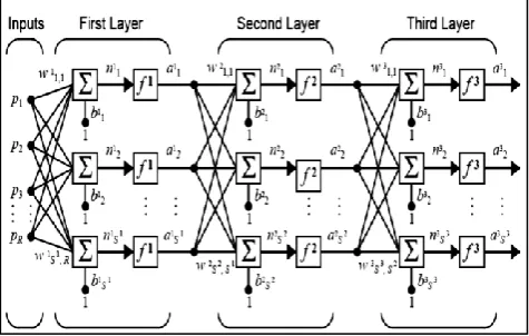
[image:2.595.314.546.67.416.2]A multilayer neural network is shown in Figure 2. Each layer has its own weight matrix W, its own bias vector b, a net input vector n and an output vector a [7]. A layer whose output is the network output is called an output layer while other layers are called hidden layers. Multilayer networks are more powerful than single layer networks. The present study implements feed-forward neural network architecture. The neural network is used to generate the tuned PID parameter values for servo motor control.
[image:2.595.314.544.72.220.2]Fig 1: Multi-layer neural network architecture
Fig 2: Neuron Model, single input and multi input neurons
Fig 3: Neuron transfer functions, hyperbolic tangent sigmoid (left) and pure linear (right)
2.2
Neural Network Algorithms
This section discusses some of the neural network algorithms used for the training of the designed neural network.
2.2.1
Levenberg-Marquardt algorithm
This algorithm was designed to approach second order training speed without having to compute the Hessian matrix [8]. When the performance function has the form of a sun of squares, then the Hessian matrix can be approximated as:
(1)
And the gradient can be computed as:
(2)
Where J is the Jacobian matrix, containing the first derivatives of the network errors with respect to the weights and biases, and e is the network error vector. The Levenberg-Marquardt algorithm uses the approximation to Hessian matrix in the following update:
(3)
[image:2.595.55.293.567.718.2]2.2.2
Bayesian regulation back-propagation
It updates the weight and bias values according to Levenberg-Marquardt optimization [9]. It minimizes a combination of squared errors and weights, and then determines the correct combination so as to produce a network that generalizes well. The process is called Bayesian regularization. Bayesian regularization minimizes a linear combination of squared errors and weights. It also modifies the linear combination so that at the end of training the resulting network has good generalization qualities. This Bayesian regularization takes place within the Levenberg-Marquardt algorithm.
2.2.3
Cyclic Order Training
This algorithm trains a network with weight and bias learning rules with incremental updates after each presentation of an input. Inputs are presented in cyclic order. For each epoch, each vector (or sequence) is presented in order to the network with the weight and bias values updated accordingly after each individual presentation.
2.2.4
BFGS quasi-Newton back-propagation
Newton's method is an alternative to the conjugate gradient methods for fast optimization. The basic step of Newton's method is:
(4)
Where, is the Hessian matrix (second derivatives) of the
performance index at the current values of the weights and biases . Newton's method often converges faster than conjugate gradient methods. Unfortunately, it is complex and expensive to compute the Hessian matrix for feed forward neural networks. There is a class of algorithms that is based on Newton's method, but which does not require calculation of second derivatives. These are called quasi-Newton (or secant) methods. They update an approximate Hessian matrix at each iteration of the algorithm. The update is computed as a function of the gradient. The quasi-Newton method that has been most successful in published studies is the Broyden, Fletcher, Goldfarb, and Shanno (BFGS) update. This algorithm requires more computation in each iteration and more storage than the conjugate gradient methods, although it generally converges in fewer iterations. The approximate Hessian must be stored, and its dimension is n x n, where n is equal to the number of weights and biases in the network.
2.2.5
Conjugate gradient algorithm
In basic back-propagation algorithm, weights are adjusted in the steepest descent direction. In the conjugate gradient algorithm, a search is performed in conjugate directions providing a faster convergence. In most of the conjugate gradient algorithms, the step size is adjusted at every iteration. All conjugate gradient algorithms start by searching in the steepest descent direction in first iteration and then perform a line search to determine the optimal distance to move along the current search direction. The next search direction is determined such that it is conjugate to previous search directions.
2.2.6
Resilient back-propagation algorithm
The use of sigmoid function in the hidden layers causes a problem in using the steepest descent to train a multilayer network. The resilient back-propagation training algorithm eliminates these effects of magnitude of the partial derivatives. The derivative sign determines the direction of the weight update. The update value of each weight and bias is increased by a factor whenever the derivative of the performance function has the same sign for two successive
iterations. The update value is decreased by a factor whenever the derivative with respect to weight changes sign from the previous iteration. The update value does not change if the derivative is zero.
2.2.7
One step secant back-propagation
Because the BFGS algorithm requires more storage and computation in each iteration than the conjugate gradient algorithms, there is need for a secant approximation with smaller storage and computation requirements. The one step secant (OSS) method is an attempt to bridge the gap between the conjugate gradient algorithms and the quasi-Newton (secant) algorithms. This algorithm does not store the complete Hessian matrix; it assumes that at each iteration, the previous Hessian was the identity matrix. This has the additional advantage that the new search direction can be calculated without computing a matrix inverse. The one step secant method is described in [10]. This algorithm requires less storage and computation per epoch than the BFGS algorithm. It requires slightly more storage and computation per epoch than the conjugate gradient algorithms. It can be considered a compromise between full quasi-Newton algorithms and conjugate gradient algorithms.
2.2.8
Scaled conjugate gradient
back-propagation
This algorithm updates weight and bias values according to the scaled conjugate gradient method but does not perform a line search at each iteration.
3.
SERVO MOTOR CONTROL
3.1
Background
In this section, speed control loop for a single phase asynchronous motor is demonstrated. The machine is fed by a PWM inverter. The speed control loop has a PID based regulator which produces a quadrature-axis current reference. The motor electromagnetic torque is controlled by this quadrature current. Hence, this method is also known as direct torque control (DTC). The motor flux is controlled by the direct-axis current. Transformation from d-q frame to a-b frame is used and the resulting currents are fed to the main and auxiliary motor windings.
The asynchronous motor has two windings: the main winding and the auxiliary winding. The electrical part of the machine is represented by a fourth order system whereas the mechanical part is represented by a second order system. The electrical parameters are referred to the stator reference frame (d-q frame). The reference frame transformation (a-b to d-q frame) is given by the following equation 5-6. The electrical behavior of the AC motor is modeled by equations 7-12, while the mechanical behavior is modeled by equations 13-14.
(5) (6)
The flux linkage equations for the direct and the quadrature axes are given by equations (3)-(8).
(9)
(10) (11) (12)
The electromechanical torque is given by
(13)
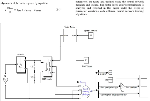
The dynamics of the rotor is given by equation
(14)
3.2
MATLAB Modeling
Neural Network design is done using the Neural Network Toolbox of MATLAB. A feed-forward back-propagation neural network is designed with 2 hidden layers of 10 neuron nodes each. Hyperbolic tangent sigmoid transfer function is used for the hidden layer nodes. The output layer uses the pure linear transfer function. A set of training data is used to train the designed neural network. A set of training algorithms are used to train the neural network and the performance of each of these is analyzed.
[image:4.595.65.562.219.553.2]The SIMULINK model for the servo motor control is shown in
Error! Reference source not found.
. Servo motor control uses the direct torque control approach. The PID parameters are tuned and updated using the neural network designed and trained. The motor speed control performance is analyzed and reported in this paper under the effect of parameter variations with different neural network training algorithms.Fig 4: SIMULINK model for servo motor control
A 0.25HP AC servo motor is used for the simulation model. The nominal motor parameters are listed in Table I.
Table 1: Nominal motor parameters
Parameter Value
Nominal Power 0.25 HP Stator resistance 2.02 ohm Stator inductance 7.4 mH
Rotor resistance 4.12 ohm Rotor inductance 5.6 mH
Inertia 0.0146 kgm2
Three different single output, multiple input neural networks are designed to be trained for tuning the proportional, integral and derivative gains of the PID controller based on the motor parameter variations. Each neural network is trained for the same set of training parameters using the gradient descent back-propagation algorithm. The advantage of training and tuning three different neural networks is that the mean square error parameter used as a performance metric is better minimized when three independent networks are tuned as compared to a single network with multiple outputs.
[image:4.595.95.253.651.768.2]different input parameter values is fed to the neural network and the neural network is trained using the gradient descent back-propagation algorithm.
4.
RESULTS AND CONCLUSION
The SIMULINK model of servo motor speed control was simulated for commanded speed of 100rpm under different loading conditions. The speed performance for un-tuned (tuning without ANN) PID parameters is shown in Fig 5. The similar speed response plot against variations in friction coefficient is shown in Fig 6.
Fig 5: Speed Response for nominal mode with different loads
Fig 6: Speed Response for different friction coefficients
4.1
Step Response
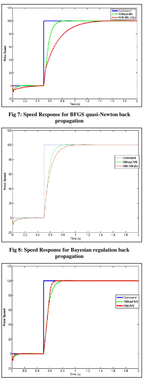
[image:5.595.314.550.66.689.2]Fig 7-Fig 13 show the speed performance for ANN tuned PID controller for the servo motor speed control. Fig 14 summarizes the speed performances for all the algorithms.
[image:5.595.52.289.188.613.2]Fig 7: Speed Response for BFGS quasi-Newton back propagation
Fig 8: Speed Response for Bayesian regulation back propagation
[image:5.595.53.288.192.380.2]Fig 10: Speed Response for Levenberg-Marquardt algorithm
Fig 11: Speed Response for one step secant back propagation
[image:6.595.315.548.73.449.2]Fig 12: Speed Response for resilient back-propagation algorithm
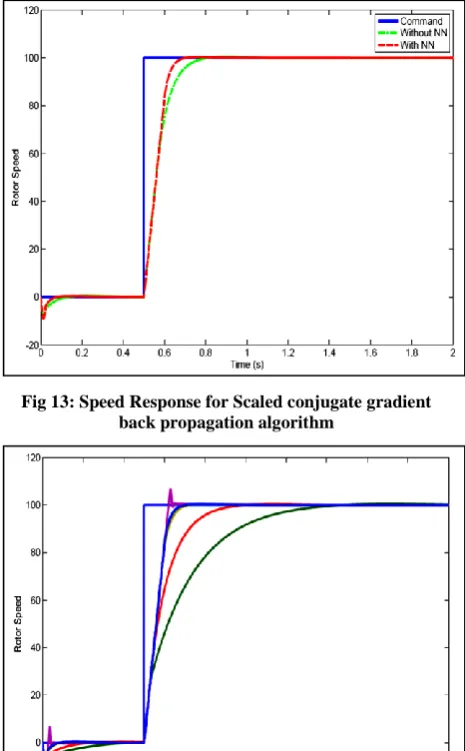
Fig 13: Speed Response for Scaled conjugate gradient back propagation algorithm
Fig 14: Speed response for different NN algorithms
It can be observed that the neural network tuning of the PID parameters improves the performance except in the case of BFGS quasi-Newton and Bayesian regulation back propagation algorithms. In all other cases the ANN tuning helps improve the response by reducing the rise time. PID tuning with Levenberg-Marquardt algorithm results in a little overshoot in the speed response. All variants of the back-propagation algorithms except the BFGS and Bayesian regulation result in a similar servo control performance. The servo performance is much improved than the gradient descent algorithm reported by Lalithamma et al [5].
4.2
Harmonic Content Analysis
[image:6.595.53.289.310.706.2]Fig 15: Command Speed profiles for harmonics study
Fig 16: Harmonic content in command torque for rectangular pulse profile
[image:7.595.313.549.68.489.2]Fig 17: Harmonic content in motor speed for rectangular pulse profile
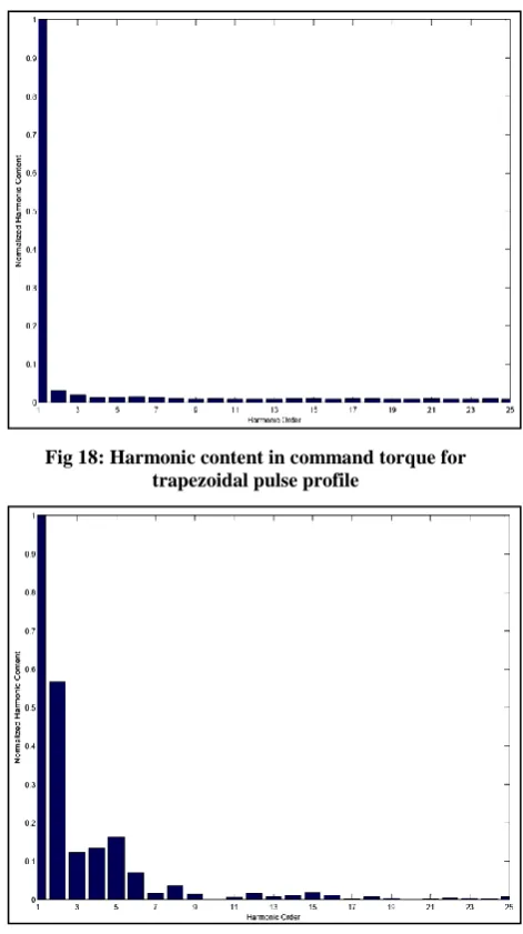
[image:7.595.60.336.72.696.2]Fig 18: Harmonic content in command torque for trapezoidal pulse profile
Fig 19: Harmonic content in motor speed for trapezoidal pulse profile
The harmonic content is higher for the rectangular speed profile as compared to the trapezoidal speed profile. The harmonic order is not affected by the neural algorithm. The applicability of neural networks for servo control applications is demonstrated. Speed control of servo motor is presented with different training algorithms. The back-propagation training algorithms are suitable for the servo motor speed control. All the back-propagation algorithms (except the BFGS and Bayesian regulation) improve the speed control performance as compared to the ones without using neural network.
5.
ACKNOWLEDGMENTS
The authors would like to express their cordial thanks to Mr Ashutosh Kumar of Planet-i Technologies for their much valued support and advice.
6.
REFERENCES
[1] A. Kaya and T. J. Scheib, “Tuning of PID controls of different structures,”Control Eng., vol. 35, no. 7, pp. 62– 65, Jul. 1988.
motor using improved self –tuning fuzzy PID controller. ICE: Annual conference in Fukui, August 4-6, 2003. [3] Pyoung-Ho kim, Sa-Hyun sin, Hyung-Lae baek,
Geum-Bae Cho, Speed control of AC servo motor neural networks.
[4] Principles of soft computing, S.N. Sivanandam , S.N. Deepa
[5] Lalithamma G A, P S Puttaswamy and Kashyap D Dhruve. Article: Multi-layer Neural Network for Servo Motor Control. International Journal of Computer Applications 71(14):32-37, June 2013. Published by Foundation of Computer Science, New York, USA [6] K.J. Hunt, D. Sbarbaro, R. Zbikowski, P.J. Gawthrop,
“Neural Networks for Control Systems: A Survey, Automatica”,pp. 1083-1122, 1992.
[7] Hagan, Martin T., Howard B. Demuth, and Mark H. Beale. Neural Network design. Boston London: Pws Pub., 1996
[8] More J J, in Numerical Analysis, Lecture notes in Mathematics 630 (Springer Verlag, Germany) 1997, 105-116
[9] Ozgur Kisi, Erdal Uncuoglu, “Comparison of three back-propagation training algorithms for two case studies”, Indian Journal of Engineering & Materials Sciences, Vol 12 Oct 2005, pp 434-442.