Mobile Position Estimation based on Three Angles of
Arrival using an Interpolative Neural Network
Omar Waleed Abdulwahhab
Computer Engineering Department, College of Engineering, University of Baghdad
ABSTRACT
In this paper, the memorization capability of a multilayer interpolative neural network is exploited to estimate a mobile position based on three angles of arrival. The neural network is trained with ideal angles-position patterns distributed uniformly throughout the region. This approach is compared with two other analytical methods, the average-position method which relies on finding the average position of the vertices of the uncertainty triangular region and the optimal position method which relies on finding the nearest ideal angles-position pattern to the measured angles. Simulation results based on estimations of the mobile position of particles moving along a nonlinear path show that the interpolative neural network approach outperforms the two other methods in its estimations for different noise conditions.
General Terms
Neural networks.Keywords
Angle of arrival (AOA), average position, optimal position, interpolative neural network.
1. INTRODUCTION
Wireless mobile positioning approaches have received a significant attention in last years. The signal being received by a mobile is used to determine its location. The mobile signal is received from several base stations with known positions. Some characteristics of that signal, such as the strength of the signal, the time of arrival of the signal, or the angle of arrival of the signal are combined with the known positions of the base stations to determine the mobile position [1]. Each characteristic defines a locus on which the mobile station must lie. For multiple measurements, the point of intersection of the corresponding loci identifies the position of the mobile station [2].
There are mainly three techniques to determine the mobile position: received signal strength (RSS) from at least three base stations, time of arrival (TOA) from at least three base stations, time difference of arrival (TDOA) from at least three base stations, and angle of arrival (AOA) from at least two base stations.
From a geometrical point of view, to locate any point in a two dimensional space (plane) specifically, it is sufficient to know either its distance from three known points, its distance from a point and its direction with respect to a point (the same first point or another point), or its directions with respect to two points.
However, due to the possible existence of non-line-of-sight (NLOS) propagation errors and measurement errors, the intersection of multiple circles (for RSS and TOA techniques) may not yield a single common point. The result is usually an
enclosed small area of uncertainty [3]. The same thing is true for angles of arrival (AOA) direction lines.
2 hybrid proposed schemes that combine time of arrival (TOA)
at three base stations and angle of arrival (AOA) at the serving base station to estimate a location of the mobile station. These schemes mitigate the NLOS effect by the weighted sum of the intersections between the TOA circles and the AOA line. An adaptive fuzzy logic estimator in a direct sequence code division multiple access (DS/CDMA) cellular system was proposed in [2]. It is based on the measured pilot signal strengths by the mobile station from several nearby base stations. A smoother that uses past and current output data from the fuzzy estimator was used to improve the accuracy of the location estimation. [12] combined the time difference of arrival (TDOA) measurements from the forward link pilot signals with the angle of arrival (AOA) measurement from the reverse link pilot signal. A two-step least square location estimator was developed based on a linear form of the AOA equation in the small error region. [13] proposed a location technique that estimates the line-of-sight (LOS) ranges based on NLOS range measurements. The approach utilizes a constrained nonlinear optimization approach for range measurements available from three base stations. The constraints were extracted from bounds on the NLOS error and the relationship between the true ranges. [14] proposed a method based on differences of downlink signal attenuations. This approach results in circles that the mobile station must lie on. The estimated mobile location is the point of intersection of these circles.
As stated in [15], there are convergence problems in the traditional Taylor series algorithm (TSA) and the hybrid lines of position algorithm (HLOP), and even if the measurements are accurate, the performance of these algorithms depends highly on the relative position of the mobile station and base stations. Therefore, they proposed an algorithm that combined both time of arrival (TOA) and angle of arrival (AOA) measurements to estimate the location of the mobile station in NLOS environments by utilizing the intersections of two circles and two lines and using the most resilient back-propagation (RPROP) neural network learning technique to estimate the location of the mobile station.
However, because of noisy measurements, it is preferable to collect data from multiple base stations in order to resolve the ambiguities resulted from multiple crossings of the lines of position and to improve the positioning accuracy [16].
2. POSITION ESTIMATION BASED ON
THREE ANGLES OF ARRIVAL
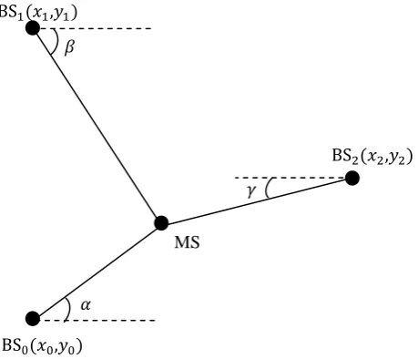
Fig. 1 shows the mobile station MS and the three closest base stations, , , and . The angles of arrival at the mobile station are , , and with respect to base stations , , and , respectively.
Equation of :
(1)
Equation of :
(2)
Equation of :
[image:2.595.320.550.72.269.2](3)
Fig. 1: Geometric layout of three angles of arrival approach
3. AVERAGE POSITION METHOD
Given the values of the three angles , , and , the mobile station position can be determined by intersecting the three lines , , and , i.e., finding the simultaneous solution of the three equations (1), (2), and (3). Ideally, the mobile station MS has consistent angles , , and , with the base stations so that the simultaneous solution of any two equations of these three equations yields the same point. However, since the angles , , and , subject to measurements errors, the three lines does not intersect at the same point. A reasonable method to estimate the mobile station position is to find the point of intersection of each two lines mutually and average the result.1) Intersection of and
(4)
2) Intersection of and
(5)
3) Intersection of and
(6)
Thus, the required point is
(7)
4. THE OPTIMAL POSITION METHOD
Equations (1), (2), and (3) can be solved for , , and , respectively in terms of and .
(8)
(9)
(10)
Considering as parameters, equations (8), (9), and (10) represent a surface in the . Each point on the surface corresponds to a point in the . However, the remaining points that do not lie on the surface do no correspond to points in the . In this paper, a noise is added to input angles; therefore in general an input point does not lie on the surface.
For a certain input , the optimization method relies on finding an absolute minimum for the cost function
which is the square of the distance between the point
and a general point on the surface . This method corresponds to that given in [17] but for AOA approach instead of TOA.
5. GENERALIZATION AND
MEMORIZATION IN AN
INTERPOLATIVE ASSOCIATIVE
NEURAL NETWORK
The interpolative associative neural network that was employed in this paper implements the mapping
where
, the i 'th stored stimuli, , the i 'th stored response.
In general, if is presented to the neural network, the output is
.
The magnitude of the vector introduces the distinction between interpolative and heteroassociative neural network. If
, it is a heteroassociative neural network, while if , it is an interpolative neural network. In this paper, generalization is required so that when a certain input that does not belong to the training pattern set is presented to the neural network, the output must be a reasonable interpolated vector. On the other hand, memorization is necessary since some input patterns have no reasonable output since they are a noisy version of the actual input vector. Here, the neural network must remember the input pattern that is closest to the distorted one, and then generalize (if this input pattern does not belong to the training set).
As is well known in such problems, over-fitting is must be avoided. However, in this paper, over-fitting was excluded by
training the neural network with ideal patterns derived from mathematical relation between position and angles of arrival.
6. ARCHITECTURE OF NEURAL
NETWORK
The neural network used in this paper is a multilayer neural network with one hidden layer. The input layer has three units which equal to the three angles of arrival at the mobile station, the hidden layer has one hundred units, and the output layer has two units which equal to the estimated coordinates of the mobile. The activation function of each neuron in the hidden layer is the unipolar sigmoid and the activation function of each neuron in the output layer is the identity function. Thus, the equation that describes this network is
,
where
is an hidden layer weight-bias matrix is a output layer weight-bias matrix is a sigmoid matrix operator
is an identity matrix operator
7. GENERATION OF TRAINING
PATTERNS
The training patterns are generated uniformly throughout the movement region. Ideal angles-position patterns are derived by finding the corresponding angles , , and for certain position using equations (8), (9), and (10). This procedure generates a set of training pattern associations
. In this paper, 400 training patterns was generated, i.e., .
8. NEURAL NETWORK TRAINING
USING ONLINE BACKPROPAGATION
ALGORITHM
The neural network was trained using online backpropagation algorithm with the previously obtained four hundred training patterns. The weight matrices and were initialized randomly. The stopping criteria was chosen based on the RMS (Root Mean Square) value of the error, defined by
where
= 400, the number of training patterns,
is the i 'th desired stored response, is the i 'th actual output.
Training of the neural network was stopped when
reaches 2. The learning rate was 0.0001 and the momentum term was 0.5. After 9009 epochs, reached 3, as shown in Fig. 2. However, it needed another 12800 epochs so that
4 Fig. 2: versus number of epochs ( =3)
Fig. 3: versus number of epochs ( =2)
9. SIMULATION RESULTS
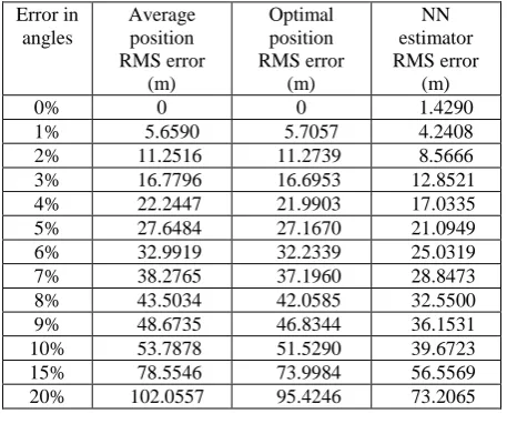
The trained neural network was used to estimate the mobile position of a particle moving along a nonlinear path described by the equation . The graph of this path is shown in Fig. 4. The neural network estimator was compared to the average position method and optimal position method. The comparison was splitted into two parts. Table 1 shows the results for the first part of the comparison for the neural network that was trained till and Table 2
shows the results for the second part of the comparison for the neural network that was trained so that reached 2. The
[image:4.595.60.292.70.253.2]comparisons were made for different angle measurement errors.
[image:4.595.319.543.75.264.2]Fig. 4: The path traced by the particle
Table 1. Comparison between average position, optimal position, and neural network estimator with
Error in angles
Average position RMS error
(m)
Optimal position RMS error
(m)
NN estimator RMS error
(m)
0% 0 0 2.1624
1% 5.6590 5.7057 4.6182 2% 11.2516 11.2739 8.9022 3% 16.7796 16.6953 13.2665 4% 22.2447 21.9903 17.5806 5% 27.6484 27.1670 21.8131 6% 32.9919 32.2339 25.9498 7% 38.2765 37.1960 29.9849 8% 43.5034 42.0585 33.9197 9% 48.6735 46.8344 37.7611 10% 53.7878 51.5290 41.5211 15% 78.5546 73.9984 59.5973 20% 102.0557 95.4246 77.2914
Table 2. Comparison between average position, optimal position, and neural network estimator with
Error in angles
Average position RMS error
(m)
Optimal position RMS error
(m)
NN estimator RMS error
(m)
0% 0 0 1.4290
1% 5.6590 5.7057 4.2408 2% 11.2516 11.2739 8.5666 3% 16.7796 16.6953 12.8521 4% 22.2447 21.9903 17.0335 5% 27.6484 27.1670 21.0949 6% 32.9919 32.2339 25.0319 7% 38.2765 37.1960 28.8473 8% 43.5034 42.0585 32.5500 9% 48.6735 46.8344 36.1531 10% 53.7878 51.5290 39.6723 15% 78.5546 73.9984 56.5569 20% 102.0557 95.4246 73.2065
10. CONCLUSIONS
[image:4.595.319.548.301.488.2] [image:4.595.58.287.302.479.2] [image:4.595.319.548.533.724.2](1) When there is no error in the measured signal characteristics, the direct analytical methods (such as average position and optimal position methods) give exactly the actual position of the mobile station while the trained neural network approximates the mobile position with some error. (2) In the presence of measurement error (due to NLOS and noise) the performance of the analytical methods begins to degrade because of the presence of the region of uncertainty while the neural network begins to exploit its memorization and generalization capabilities to handle this region. Therefore, as the percentage error of the angles measurements increases, the neural network begins to outperform the geometrical methods. (3) For the two versions of the neural network ( and
), the second one outperforms the first as it is
obvious . The reason is that continuously training the network does not encounter an over-fitting problem because it was trained with ideal training patterns.
11. REFERENCES
[1] Karray, F. O. and Silva, C. D. (2004) Soft Computing and Intelligent Systems Design. England: Pearson education.
[2] SHEN, X. MARK, J. W. and YE, J. (2002) Mobile Location Estimation in CDMA Cellular Networks by Using Fuzzy Logic. Wireless Personal Communications. [online] vol. 22(1). P. 57-70. Available from: www.ivsl.org [Accessed: 10th April 2014].
[3] Wann, C. and Chen, Y. (2002) Position Tracking and Velocity Estimation for Mobile Positioning Systems. In- Wireless Personal Multimedia Communications. vol. 1. p. 310-314. Available from: www.ivsl.org [Accessed: 10th April 2014].
[4] Caffery, J. and St¨uber, G. L. (1998) Subscriber Location in CDMA Cellular Networks. IEEE Transactions on Vehicular Technology. [online] vol. 47(2/May). P. 406-416. Available from: www.ivsl.org [Accessed: 10th April 2014].
[5] Wei, K. and Lenan, W. (2009) Constrained Least Squares Algorithm for TOA-Based Mobile Location under NLOS Environments. In- 5th International Conference on Wireless Communications, Networking and Mobile Computing. P. 1-4. Available from: www.ivsl.org [Accessed: 10th April 2014].
[6] Yang, C., Chen, B. and Liao, F. (2010) Mobile Location Estimation Using Fuzzy-Based IMM and Data Fusion. IEEE Transactions on Mobile Computing. [online] vol. 9(10/October). p. 1424-1436. Available from: www.ivsl.org [Accessed: 10th April 2014].
[7] LiuYing, Liang,Y., and Wang, S. (2000) Location Parameters Estimation in Mobile Communication Systems. In- Communication Technology proceeding. vol. 1. p. 261-268. Available from: www.ivsl.org [Accessed: 10th April 2014].
[8] Voltz, P. J. and Hernandez, D. (2004) Maximum Likelihood Time of Arrival Estimation for Real-Time Physical Location Tracking of 802.1 1 a/g Mobile Stations in Indoor Environments. In- Position Location
and Navigation Symposium. p. 585-591. Available from: www.ivsl.org [Accessed: 10th April 2014].
[9] Chen, C. and Feng, K. (2005) Hybrid Location Estimation and Tracking System for Mobile Devices. In- IEEE 61st Vehicular Technology Conference. vol. 4. p. 2648-2652. Available from: www.ivsl.org [Accessed: 10th April 2014].
[10]Zhou, J., Chu, K. M., and Ng, J. K. (2009) A Probabilistic Approach to Mobile Location Estimation within Cellular Networks. In- 15th IEEE International Conference on Embedded and Real-Time Computing Systems and Applications. P. 341-348. Available from: www.ivsl.org [Accessed: 10th April 2014].
[11]Chen, C., Su, S., and Lu, C. (2010) Geometrical Positioning Approached for Mobile Location Estimation. In- 2nd IEEE International Conference on Information Management and Engineering. p. 268-272. Available from: www.ivsl.org [Accessed: 10th April 2014].
[12]Cong, L. and Zhuang, W. (2002) Hybrid TDOA/AOA Mobile User Location for Wideband CDMA Cellular Systems. IEEE Transactions on Wireless Communications. [online] vol. 1(3/July). p. 439-447. Available from: www.ivsl.org [Accessed: 10th April 2014].
[13]Venkatraman, S., Caffery, J. and You, H. (2004) A Novel ToA Location Algorithm Using LoS Range Estimation for NLoS Environments. IEEE Transactions on Vehicular Technology. [online] vol. 53(5/September). p. 1515-1524. Available from: www.ivsl.org [Accessed: 10th April 2014].
[14]Lin, D. and Juang, R. (2005). Mobile Location Estimation Based on Differences of Signal Attenuations for GSM Systems. IEEE Transactions on Vehicular Technology. [online] vol. 54(4/July). p. 1447-1454. Available from: www.ivsl.org [Accessed: 10th April 2014].
[15]Chen, C. and Lin, J. (2011) Applying Rprop Neural Network for the Prediction of the Mobile Station Location. Sensors. [online] vol. 11(4). p. 4207-4230. Available from: www.ivsl.org [Accessed: 10th April 2014].
[16]Landolsi, M. A., Muqaibel, A. H. , Al-Ahmari, A. S. , Khan, H.-R. and Al-Nimnim, R. A. (2010). Performance Analysis of Time-of-Arrival Mobile Positioning in Wireless Cellular CDMA Networks. In- Bouras, C. J. (ed.). Trends in Telecommunications Technologies.
[online] Available from:
http://www.intechopen.com/books/trends-in- telecommunications-technologies/performance-analysis- of-time-of-arrival-mobile-positioning-in-wireless-cellular-cdma-networks. [Accessed: 10th April 2014].
[17]Liu, H. Darabi, H. Banerjee, P. and Liu, J. (2007) Survey of Wireless Indoor Positioning Techniques and Systems. IEEE Transactions on Systems, Man, and Cybernetics—Part C: Applications and Reviews. [online] vol. 37(6/November). Available from: www.ivsl.org [Accessed: 10th April 2014].