Computer Science Theses Department of Computer Science
5-9-2015
FPGA Based Binary Heap Implementation: With
an Application to Web Based Anomaly
Prioritization
Md Monjur Alam
Follow this and additional works at:https://scholarworks.gsu.edu/cs_theses
This Thesis is brought to you for free and open access by the Department of Computer Science at ScholarWorks @ Georgia State University. It has been accepted for inclusion in Computer Science Theses by an authorized administrator of ScholarWorks @ Georgia State University. For more information, please [email protected].
Recommended Citation
Alam, Md Monjur, "FPGA Based Binary Heap Implementation: With an Application to Web Based Anomaly Prioritization." Thesis, Georgia State University, 2015.
WEB BASED ANOMALY PRIORITIZATION
by
MD MONJUR ALAM
Under the Direction of Sushil K. Prasad, PhD
ABSTRACT
This thesis is devoted to the investigation of prioritization mechanism for web based
anomaly detection. We propose a hardware realization of parallel binary heap as an
appli-cation of web based anomaly prioritization. The heap is implemented in pipelined fashion in
FPGA platform. The propose design takesO(1) time for all operations by ensuring minimum
waiting time between two consecutive operations. We present the various design issues and
hardware complexity. We explicitly analyze the design trade-offs of the proposed priority
queue implementations.
WEB BASED ANOMALY PRIORITIZATION
by
MD MONJUR ALAM
A Dissertation Submitted in Partial Fulfillment of the Requirements for the Degree of
Master of Science
in the College of Arts and Sciences
Georgia State University
WEB BASED ANOMALY PRIORITIZATION
by
MD MONJUR ALAM
Committee Chair: Sushil K. Prasad
Committee: Xioajun Cao
Yanqing Zhang
Electronic Version Approved:
Office of Graduate Studies
College of Arts and Sciences
Georgia State University
DEDICATION
ACKNOWLEDGEMENTS
This dissertation work would not have been possible without the support of many people.
I want to express my gratitude to my advisor Dr Sushil K. Prasad, for providing me an
opportunity to work on this thesis. He has been guiding me through all the obstacles
encountered in my research work and has been a constant source of motivation.
I must extend my thanks to all the committee members of this thesis, Dr. Xiaojun Cao
and Dr. Yanqing Zhang, for there valuable suggestions to help in shaping this thesis.
There is a substantial contribution made by my wife Tazneem Alam to help me to finish
this work. Apart from helping figure drawing, she has been the constant source of motivation
in my ups and downs carrier. I must extend my thanks to her for providing healthy and
tasty food through out my MS tenure.
I should not ignore the help of one innocence, my three year angel, Afnan Alam. While
I am fatigue with work pressure, frustrated with the outcomes of research works; playing
and giving accompany to this little baby boy alleviate my mental pain and these come to
TABLE OF CONTENTS
ACKNOWLEDGEMENTS . . . v
LIST OF TABLES . . . viii
LIST OF FIGURES . . . ix
LIST OF ABBREVIATIONS . . . x
PART 1 INTRODUCTION . . . 1
1.1 Motivation of the Work. . . 1
1.2 Objective and Design Issues . . . 2
1.3 Main Contribution . . . 2
1.4 Organization of the Thesis . . . 3
PART 2 PRELIMINARY AND RELATED WORK . . . 4
2.1 Web Based Anomaly . . . 4
2.1.1 Score Calculation . . . 4
2.1.2 Prioritization . . . 5
2.2 Priority Queue . . . 6
2.2.1 Priority Queue Implementation . . . 6
2.3 Related Work . . . 8
2.3.1 Anomaly Detection by Using Hardware . . . 9
2.3.2 Parallel Priority Queue . . . 9
PART 3 FPGA BASED PARALLEL HEAP . . . 12
3.1 Insert Operation . . . 12
3.2 Delete Operation . . . 14
3.4 Pipeline Design . . . 19
3.4.1 Optimization Technique . . . 20
3.5 Implementation Result . . . 23
3.5.1 Hardware Cost . . . 25
PART 4 CONCLUSIONS AND FUTURE WORK . . . 26
4.1 Future Scope of Work . . . 26
REFERENCES . . . 28
APPENDICES . . . 33
Appendix A SOURCE CODE . . . 33
LIST OF TABLES
Table 3.1 Variation of frequency, execution time and throughput with number
of level . . . 23
LIST OF FIGURES
Figure 2.1 Illustrating anomalies in a two-dimensional data set [26]. . . 4
Figure 2.2 Markov Model Example [40]. . . 5
Figure 2.3 Binary Min Heap. . . 6
Figure 2.4 Array Representation of Binary Min Heap. . . 6
Figure 2.5 New heap structure after insertion 18. . . 7
Figure 2.6 New heap structure after single deletion operation from the original heap shown at figure 2.3. . . 8
Figure 3.1 Storage in FPGA of deferent nodes in binary heap . . . 12
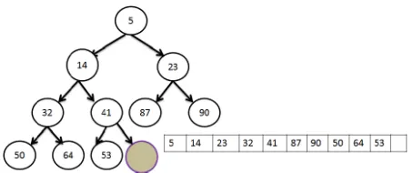
Figure 3.2 Insertion path . . . 13
Figure 3.3 Contain of latch (L) after insertion completed . . . 13
Figure 3.4 Hole is the resultant for parallel operation of insert-delete . . . 15
Figure 3.5 Contain of latch (L) after parallel operation of insert-delete . . . . 15
Figure 3.6 Top Level Architecture of insert-delete . . . 16
Figure 3.7 Pipeline Design Overview . . . 19
Figure 3.8 Parallel insert operation: illustrates operations at each level at each clock . . . 20
Figure 3.9 Parallel delete operation: illustrates operations at each level at each clock. . . 21
Figure 3.10 Sharing Insert-Deletehardware resulting reducing combinational logic by half . . . 22
Figure 3.11 Different performance matrices . . . 24
Figure B.1 Print screen of simulation out put . . . 50
LIST OF ABBREVIATIONS
• GSU - Georgia State University
• CS - Computer Science
• FPGA - Field Programmable Gate Array
PART 1
INTRODUCTION
Anomaly detection refers to the problem of finding patterns in data that do not conform
to a well defined notion of normal behavior. We often refer these nonconforming patterns as
anomalies or outliers [26]. Network based anomaly detection deals with score calculation and
prepares a ranking for all packets based on that score. Due to high network congestion, it is
incumbent to provide an efficient interface that can handle prioritization of packets based on
the score assigned. As software based application inherently provides slower interface, the
hardware based prioritization interface is necessary. Based on the priority, the interface will
take some decisions (either pass or drop). For a high speed traffic, it is required to process
these tasks in parallel.
Implementation of parallel priority queue will solve this requirement. A priority queue
(PQ) is a data structure in which each element has a priority and a dequeue operation
removes and returns the highest priority element in the queue. PQs are the most basic
component for scheduling, mostly used in routers, event driven simulators [17], etc. There
are several hardware based PQs implementations that are usually implemented by either
ASIC chips [8,9,15] or FPGA [17-19]. But, all of them suffer some limitations and not
applied to all applications.
1.1 Motivation of the Work
In the literature, several hardware-based priority queue architectures have been
pro-posed [14,15]. All of these schemes have one or more shortcomings. The Systolic Arrays
andShift Registers based approaches [14,15], for example, are not scalable and require much
hardware, more specifically, it requireO(n) comparators fornnodes. FPGA based pipelined
run for 64K nodes without compromising performance. The major drawback of this design
is that it takes at least 3 clock cycles to complete a single stage. More over, it never address
theholegenerated by paralleldeleteoperation followed by aninsertion. The calendar queues
implemented by [8] can only accommodate a small fixed set of priority values since a large
priority set would require extensive hard-ware support.
1.2 Objective and Design Issues
The objective of this work is to find a suitable design of parallel priority queue on
FPGA platform to provide an efficient interface for the anomaly detector engine to handle
packets prioritization very fast. We will store data based on its priority and this will be
possible by incorporating parallel addition operation in binary heap. To access the highest
priority data, we need to implementdeleteoperation from the binary heap. Let us implement
minimum (min) binary heap where root contains the maximum (max) priority element. As
our intention is to provide efficient interface, the following design issues we should address
while implementing it.
• To minimize waiting time for two consecutive operations.
• To minimize hole created by deletion.
• The design should be highly scalable and optimized.
1.3 Main Contribution
We have implemented a software based anomaly detection mechanism where a score
is assigned to each packet. We apply Markov based model for score calculation. A FPGA
based parallel binary heap is implemented for score prioritization. We present the various
design issues and hardware complexity. The pipeline architecture ensures no waiting time
for any operation except thedeletionone which has to wait for a single cycle. Each ofinsert
priority queue implementations. Our design takes care the hole created bydelete operation.
We minimize the hole at the time of insertion.
1.4 Organization of the Thesis
A Summary of the contents of the chapters to follow is given below:
Part 2: Contains an overview and the art of literature related to the work.
Part 3: Our proposed design including implementation result is presented here. We also
describe different design trade-off in this part.
Part 4 : This part contains some concluding remarks and identifies some directions for
PART 2
PRELIMINARY AND RELATED WORK
2.1 Web Based Anomaly
Figure (2.1) Illustrating anomalies in a two-dimensional data set [26].
Anomaly detection refers to the problem of finding patterns in data that do not conform
to a well defined notion of normal behavior. We often refer these nonconforming patterns as
anomalies or outliers. Fig. 2.1 depicts anomalies in a simple two-dimensional data set [26].
There are two normal regionsN1 and N2 for the data since most observations reside in these
regions. The points o1 and o2 and all the points in region O3 are considered as anomalies
as theses points are sufficiently far away from the two normal regions. We can consider net
work packet in each region as data set. Each packet belongs to a particular set based on its
score calculation.
2.1.1 Score Calculation
Among several methods, Markov model is one to calculate score for each packets [40].
The Markov model (MM) can be viewed as a probabilistic finite state automaton (PFSA)
which generates sequences of symbols. The output of the Markov model consists of all
[image:16.612.235.373.228.350.2]Figure (2.2) Markov Model Example [40].
output transition and the resultant score is calculated as the summation of all transition
probability. For example, consider the non-deterministic finite automata (NFA) in Figure
2.2. To calculate the probability of the word ‘ab’, one has to sum the probabilities of the
two possible paths (one that follows the left arrow and one that follows the right one). The
start state emits no symbol and has a probability of 1. The result is
p(w) = (1.0∗0.3∗0.5∗0.2∗0.5∗0.4) + (1.0∗0.7∗1.0∗1.0∗1.0∗1.0)
= 0.706 (2.1)
2.1.2 Prioritization
Software based score prioritization of network packets are presented by Kruegel et. al
[24]; where the packets with maximum score gets high priority to be processed next. Each
time, score is calculated on the fly and it is compared with other set of precalculated scores.
Effectively, there is a processing delay to come up with a decision. Moreover, processing
parallel packet is not possible here, as the on the fly calculation here is highly serialized
[image:17.612.244.370.78.229.2]2.2 Priority Queue
A priority queue is an abstract data structure that maintains a collection of elements
with the following set of operations by a minimum priority queueQ:
• Insert: A number ni is inserted into the set of candidate number N in Q, provided
that the new list maintain the priority queue.
• Delete: Find out the minimum number in Qand delete that number fromQ. Again, after deletion the property of priority queue should be kept unchanged.
Figure (2.3) Binary Min Heap.
Figure (2.4) Array Representation of Binary Min Heap.
2.2.1 Priority Queue Implementation
Priority queue can be implemented by using binary heap data structure.
Definition 2.2.1 A min-heap is a binary tree H such that (i) the data contained in each node is less than (or equal to) the data in that nodes children and (ii) the binary tree is
[image:18.612.191.418.441.536.2]Figure 2.3 shows the binary min heap (H). The root of H is H[1], and given the index
iof any node in H, the indices of its parent and children can be determined in the following
way:
parent[i] = bi/2c
lef tChild[i] = 2i rightChild[i] = 2i+ 1
Figure 2.4 illustrates the array representation of binary heap. The insertion algorithm
on the binary min heap H is as follow:
• Place the new element in the next available position (say i) in theH.
• Compare the new element H[i] with its parent Hbi/2c. If H[i] < Hbi/2c, then swap
it with its parent.
• Continue this process until either (i) the new elements parent is smaller than or equal
to the new element, or (ii) the new element reaches the root (H[1]).
Figure (2.5) New heap structure after insertion 18.
Figure 2.5 shows the new heap structure after insertion of 18 at the heap presented in
Figure 2.3.
The deletion algorithm is as follow:
[image:19.612.234.377.465.573.2]Figure (2.6) New heap structure after single deletion operation from the original heap shown at figure 2.3.
• Replace the rootH[1] by the last element at the last level (say H[i]).
• Compare root with its children and replace the root by its min child.
• Continue this replacement for each level by comparing H[i] with H[2i] and H[2i+ 1],
un till the parent become less than its children or it reaches to the leaf node.
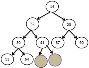
Figure 2.6 depicts the heap structure of single deletion operation from the original heap
shown at Figure 2.3. We can see that 5 was the root element at Figure 2.3. The updated
Figure 2.6 depicts that the 5 is no anymore after thedeletion. Moreover, heap is re-structured
according to the deletionalgorithm presented above.
2.3 Related Work
Many web anomaly detection techniques have been proposed which applied a set of
training data to define a model of normal behaviour. It labelled any data as abnormal that
is not included in this model [25,27,29,31,35-37]. Several variants of the basic technique
[image:20.612.234.378.69.180.2]have been proposed for network intrusion detection, and for anomaly detection in text data
[23,34,39]. These approaches assume independence between the different attributes. Some
approaches have been introduced that assume the conditional dependencies between the
dif-ferent attributes applying more complex Bayesian networks [28,33,38]. Rule-based anomaly
detection techniques distinguish normal behavior of data instances from anomalies by
are two steps for rule-based anomaly detection approach. First, rules are learned from the
training data using a rule learning algorithm. A confidence value is associated with every
rule. The second step is to search the rule that best captures the test data instance. The
anomaly score of the test instance is calculated as the inverse of the confidence associated
with the best rule. For example, a typical rule-based system is an expert system where the
rules are generated by humans [26,30,32].
All of the approaches mentioned suffer from two basic problems:
1. There is no efficient implementation to deal with huge network congestion.
2. prioritization of network traffic is not maintained.
2.3.1 Anomaly Detection by Using Hardware
To resolve the first class of difficulty several authors [20,22] come up with hardware based
solution. The intention is to provide very fast interface to process network data. To achieve
this goal, Das et. al. [20,21] comes up with hardware based solution for anomaly detection.
The work comprises of a new Feature Extraction Module (FEM) which summarizes the
network behavior. It also incorporates an anomaly detection mechanism using Principal
Component Analysis (PCA) as the outlier detection method. The authors of [22] propose a
mechanism of feature extraction. The method is implemented on FPGA and it is suitable
for large network with high data flow.
2.3.2 Parallel Priority Queue
Several authors have theoretically proved that parallel heap is an efficient data structure
to implement priority queue. Prasad et. al. [1,4] theoretically illustrate this data structure
to show O(p) operations are required with O(logn) time forp ≤ n, where n is the number
of nodes and p is the number of processor used. The idea is designed for EREW PRAM
shared memory model of computation. The many core architecture by [3] in GPGPU
processing time for n number of nodes. The implementation of this algorithm is expensive for multi-core architectures [6].
Hardware Based Priority Queue There have been several hardware based parallel
priority queue implementations described in the art of literature [8-15]. Pipelined based
ASIC implementations can reach O(1) execution time [11,12]. Due to several limitations
like cost and size, most of the ASIC implementations does not support a large number of
nodes to be processed. These implementation are also limited to high scalability. In [13],
the author claims the pipelined heap presented be the most efficient one. However, this
implementation incurs high hardware cost. The design is not flexible, more specifically, it is
designed with a fixed heap size. The Systolic Arrays and the Shift Registers [14,15] based
hardware implementations are well known in the literature. The common drawback of these
two implementation is using a large number of comparator (O(n)). The responsibility of
comparators used here to compare nodes in different level with O(1) step complexity. For
the shift register [15] based implementations, when new data comes for processing, it is
broadcasted to all levels. It requires a global communicator hardware which can connect
with all level. The implementation based on Systolic Arrays [14] needs a bigger storage
buffer to hold pre-processed data. These approaches are not scalable and require much
hardware, more specifically, it require O(n) comparators for n nodes. To overcome the
hardware complexity, a recursive processor is implemented by [16]; where a drastic hardware
is reduced by compromising execution timing cost. Bhagwan and Lin [9] designed a physical
heap such a way that commands can be pipeline between different levels of heap. The authors
in the paper [8] give some pragmatic solution of so calledfanout problem mentioned in [10].
The design presented in [41] is very efficient in terms of hardware complexity. But, as the
design is implemented by using hardware-software co-design, it is very slow in execution
(O(logn)).
For the FPGA based priority queue implementation, Kuacharoen et. al [19]
to be acted as a task scheduler in real time. The major limitation of this paper is that it
deals with very small number of nodes. A hybrid priority queue is implemented by [18] and
it ensures high scalability and high throughput. FPGA based pipelined heap is presented
by Ioannou et. al [17]. This architecture is very much scalable and can run for 64K nodes
without compromising performance. The major drawback of this design is that it takes at
least 3 clock cycles to complete a single stage. More over, it never address theholegenerated
PART 3
FPGA BASED PARALLEL HEAP
Like an array representation, heap can be represented by hardware register or FPGA
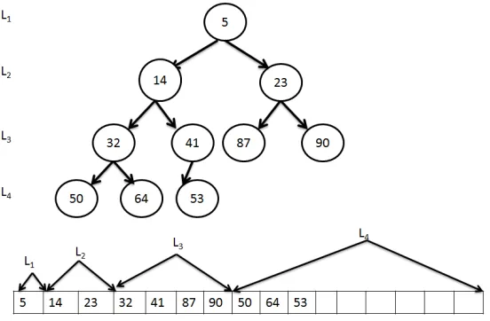
latch. Each level of the heap can be virtually represented by each latch. The size of the
latch at each level can be represented as 2β−1, whereβ is the level assuming that root is the
level 1. Figure 3.1 shows the different latches do represent the different levels. Here, root
node can be stored by L1, the next level with two elements can be stored inL2 and the last
level with 3 elements can be stored in L4, although the last level can have max 8 elements.
Figure (3.1) Storage in FPGA of deferent nodes in binary heap
3.1 Insert Operation
We have already discuss the insert operation which is intimated from the last available
node of the heap. This bottom up approach restrict the other operations like delete, replace,
etc. to perform in parallel. As deletion means the least element to be deleted and the least
element always resides at root in case of min heap; deletion operation should wait till the
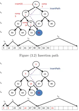
[image:24.612.169.445.326.507.2]Figure (3.2) Insertion path
Figure (3.3) Contain of latch (L) after insertion completed
Figure 3.1, followed by delete one element from heap then what will happen? Let us assume
nodes at each level get updated by a single clock cycles. That means, in worst case, total
4 clock cycles are required to complete the insert operation in this situation. So, delete
operation either has to wait for 4 clock cycles or it will wrongly delete the root, which is 5.
So, it is incumbent to insert from root and go down. But, we need to know the path for the
new inserted element, otherwise the tree will not be complete binary tree. We have adopted
a nice algorithm presented by Vipin et. al [7] in our design. The algorithm is as follow:
• Letk is the last available node at where new element to be inserted. Let j be the first
[image:25.612.169.447.67.456.2]• Let k−j = B, which binary representation is bβ−1bβ−2· · ·b2b1. Starting from root,
scan each bit of B starting from bβ−1;
– if bi == 0 (i∈ {β−1, β−2,· · · ,2,1), then go to left
– else go right
The Figure 3.2 shows the insertion path for new element to be inserted. For the new
element insertion, node at 11 should be filled up. The first node of the last level is at index
8. So, 11-8 = 3, which can be represented as 011. So, starting from root, the path should
be root→lef t→right→right and this can be demonstrated by the Figure 3.2. After the insertion completion, the contain of the nodes along with the value of latch is presented by
the Figure 3.3.
3.2 Delete Operation
There is one conventional approach to delete element from heap. As root resides the
min element, deletion always happen from root and the last element is replaced to root.
There are two difficulties here:
1. For sequential operation, it works perfectly file. For, parallel execution of insert/del,
hole can be created here. The situation happen after any insert followed by delete
operation.
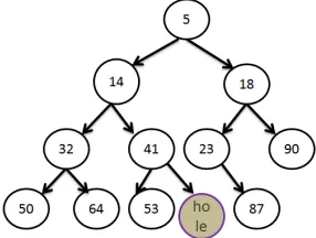
From the Figure 3.4 we can illustrate this scenario clearly. Let at t1, the operation
insert with element 100 is encountered and it is denoted byinsert(100). Obviously, the
element will be inserted at the last node of last level which is 12. Let, after one clock
cycle ofinsert, deleteis encountered (say at t2). At, that time, insert was modifying
at L2. So, due to delete, hole will be created at node 10th as shown in Figure 3.4.
Eventually, when insert(100) will finish, the element 100 will occupy at the position
of H[12], but, H[11] will become empty. This situation is illustrated by Figure 3.5.
Let us assume that insert instruction comes at time ti and delete instruction comes
Figure (3.4) Hole is the resultant for parallel operation of insert-delete
Figure (3.5) Contain of latch (L) after parallel operation of insert-delete
one clock cycle at any level to complete tasks at that level. It is obvious that, only
single node gets modified (if any) for all levels. In general, for any insert−delete
combination, hole will be created if (tj−ti)< β, whereβ is the depth of heap.
2. While you replace root by last element of heap, it requires extra clock cycle. Moreover,
we need to compare three elements, root and its two children or any node and its
children. For hardware perspective, it is cost efficient to compare two elements rather
than to compare three elements. More over, it incurs the path delay longer.
So, we should intentionally avoid the root replacement by last element. Let us delete
[image:27.612.170.441.68.244.2] [image:27.612.170.441.280.454.2]this case, we can save one cycle and hardware cost, more specifically, can minimize the path
delay. Now, our aim is to minimize hole by adding logic.
3.3 Insert-Deletion Logic Implementation
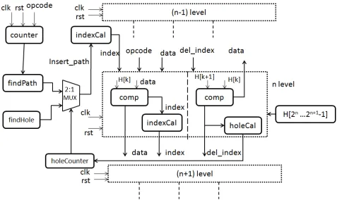
Figure (3.6) Top Level Architecture of insert-delete
Figure 3.6 illustrates the top level architecture ofinsertion-deleteoperation. Thecounter
is used to maintain the total number of element present in the heap. It is incremented by
one for insertoperation and decremented by one for deletion operation. The indexCal block
is used to find the insertion path. We have modified the existing path finding algorithm by
[7]. We first consider the holeReg to obtain insertion path. The holeReg contains the holes
created atdeletionoperation. We maintain a holeCounterto identify a validhole. Based on
the index, the heap node is accessed and the node is compared with the present data. Based
on the comparison, either the node is updated by present data and the node is passed to the
[image:28.612.78.555.189.473.2]the next level.
Deletion : We maintaindel index to find the last deleted node. For example, initially,
del index becomes 1 which means root is deleted. The comparator finds the min element
betweenH[del index∗2] andH[del index∗2 + 1] and that min gets replace to H[del index].
Now,del index gets modified with the index of min element. Again the comparator finds the
min of the ancestors of the new index and replace the node of new index with that of min
one. Each time holeCal finds if there is a valid child for del index. If there is no valid child,
then holeCounter is incremented by 1 and holeReg is updated with del index. By this way,
we maintain hole.
Algorithm 1 Algorithm for Insert−Delete(data, opcode)
1: if (opcode == 1) then
2: counter = counter +1;
3: if (holeCounter >0) then
4: insert path = f indP ath(counter, holeCounter)
5: end if
6: for (0to number of level) do
7: index =indexCal(insert path)
8: if (data < H[index] then 9: H[index] =data
data=H[index]
10: else
11: data=data 12: end if
13: end for 14: else
15: Remove H[1]
16: while (lef tChild[del index]6=N U LL&rightChild[del index]6=N U LL)do 17: if (lef tChild[del index]< rightChild[del index]) then
18: H[del index] =lef tChild[del index]
del index=del index∗2
19: else
20: H[del index] =rightChild[del index]
del index=del index∗2 + 1
21: end if 22: end while
23: hole counter =hole counter+ 1
hole reg[hole counter] =del index
Theinsert-deleteparallel algorithm is presented at Algorithm 1. We use 2:1 multiplexer
to select the path based on the value of holeCount. The logic for findPath is illustrated at
Algorithm 2. The indexCal block is implemented based on the value of findPath and the
logic is illustrated at Algorithm 5. To calculate the first node of last level is noting but the
mathematical expression of 2β−1 where β is the level of heap. There is some difficulty to
realize this expression in hardware. We express this logic by Algorithm 3.
Algorithm 2 Algorithm for f indP ath(counter, holeCounter)
1: if (holeCounter >0)then 2:
3: return f indHole(holeCounter)
4: else
5: leaf node = f ind 1st node last level(counter)
6: return (counter−leaf node
7: end if
Algorithm 3 Algorithm for f ind 1st node last level(counter)
1: for (i = 0; 2i < counter; i = i+1) do
2: leaf node = i+1
3: end for
4: return leaf node
Algorithm 4 Algorithm for f indHole(hole counter)
1: return holeReg[holeCounter]
We have used global clock(clk) and global reset(rst) signal for the each logic block except
the combinational logic parts. The clk and rst signals are not mentioned at each figure due
to place limitation. The function offindHole is basically an implementation of stack register
Algorithm 5 Algorithm for indexCal(insert path)
1: for (i = 0 to insert path bits) do
2: if (bit == 0) then
3: indexi = 2*index(i−1)
4: else
5: indexi = 2*index(i−1) + 1
6: end if 7: end for
Figure (3.7) Pipeline Design Overview
3.4 Pipeline Design
To achieve high throughput we need to start one operation before completing the
previ-ous operation. So, many operation can be in progress in the tree. To achieve so, we consider
our design to take a single clock cycle to perform each stage. For any stage, only one
opera-tion (insert, delete) can be execute at ant timet. That is why we need all operation should
be started from the top (root) of the tree and proceed towards the bottom (leaf).
[image:31.612.92.513.160.475.2]perform insertion or deletionbased on the signalopcode. Each level takes three clock cycles
to perform all operations. Each level sends data and opcode to the next level to perform.
There is a global clock and global reset attached to each stage. All the level contains the
same logic hardware except the first level.
3.4.1 Optimization Technique
Figure (3.8) Parallel insert operation: illustrates operations at each level at each clock
We need to know the operations at each level at each clock cycle to provide more
optimization. We make each individual operations like Read, Write and compare (comp) to
complete in separate single clock cycle. Each level has to perform these three basic operations
resulting three clock cycles in total. We pre-compute data for a level such a way that there
are maximum overlap between consecutive two levels in case of insertion. For any level β,
if Read operation executes at t time, then it executes comp operation at t+ 1. The comp
generates the nextindex to be read by the next level. So,β+ 1st level perform Readatt+ 1
time. Now, β level performs write operation at t+ 2, while β+ 1st level finish comp and
generates the index to be read by theβ+2ndlevel. At timet+3, theβ+1st level will perform
[image:32.612.83.521.217.442.2]available for theβ+3rdlevel. By this ways, we find there are two operations overlaps between
two consecutive levels in 3 cycles. Effectively, it results of writing at each clock cycle after
initial latency of two clock cycle at the first level. The Figure 3.8 illustrates this situation.
We can see that, while level L2 perform comp at clock 2, then level L3 performs the Read.
The levelL2completesWriteat clock 3, while levelL3 completes thecompfollowed byWrite
at clock 4. We make comp operation by β and Read operation by β+ 1 at same clock cycle
t by using the concept of different edge of clock. Level L2, for example, performs comp at
positive edge of clock 2 and level L3 performs Read at negative edge of clock 2.
Figure (3.9) Parallel delete operation: illustrates operations at each level at each clock.
Hardware Sharing Unlike, theinsert, thedeleteoperation of any level waits for data
from its next level. As the min element of a certain levels go up to the upper level, the data
will be available to write after performing the comp operation of that level. In general, if
Readoperation executes atttime by levelβ, then it executescomp operation att+ 1 (except
root level). As the comp generates the next index to be read by the next level. So, β+ 1st
level perform Readat t+ 1 time. But, the level β can not perform Write operation att+ 2,
[image:33.612.85.532.283.510.2]Figure (3.10) Sharing Insert-Delete hardware resulting reducing combinational logic by half
byβ+ 1st level will be available after t+ 2; that means the level β can performWrite only
at time t+ 3. Att+ 2 the levelβ becomes idle. For each level, we can see that there is such
idle state. For example, while level L2 perform comp at clock 2, then level L3 performs the
Read (Figure 3.9). Level L2 becomes idle at clock 3 while L3 performs comp at that time.
Eventually, the level L2 performs Write at clock 4 after the data available by the level L3
performs. From the Figure 3.9, we can see that at clock 3 the data fromL2is written at level
L1. That means, the level L2 suffers at a temporary hole at clock 3. This hole at level L2
is compensated while the level L3 write at L2 at clock 4. But, the the level L3 suffers from
temporary hole. While a level has temporary hole, the level is in inactive state; that means
there could not be any operation to be performed at that level at that time. In general, for
any timet, theβ level can not be completed if β+ 1 level can not finish the task ofcomp at
t+ 1. That means we can share hardware between the levels β and β+ 1.
Figure 3.10 illustrates the hardware sharing where a commonInsert-Deleteblock is used
[image:34.612.130.488.77.330.2]Table (3.1) Variation of frequency, execution time and throughput with number of level
Number of Level Frequency (f) Execution Time Throughput (τ)
(β) (MHz) (ns) (GB/Sec)
4 318.8 9.41 1.27
8 232.8 12.88 1.85
10 212 14.15 2.12
12 210 14.25 2.52
16 207.2 14.5 3.31
20 173.4 17.3 3.46
24 171.6 17.48 4.10
28 157.45 19.05 4.39
32 143.69 20.87 4.57
3.5 Implementation Result
The proposed design has been simulated by ISim for implementation on Xilinx Sparttan6
XC6SLX4 hardware platform.
(τ) is calculated as:
τ = ω×f
χ (3.1)
whereωis the bit length,f is the clock frequency andχis the number of clock cycle required
to computeinsert-delete. We obtain maximum clock frequency of 207.21 MHz with minimum
clock period of 4.82 nano second (ns).
Table 3.1 demonstrates the performance result obtained from simulation. The execution
time per level is calculated as:
t = 3
f (3.2)
where β is the number of level and f is the frequency. We use the number of level (β)
[image:35.612.122.492.106.271.2]Form the table, we found that the obtained clock frequency is not constant, it is inversely
proportion to the bit length (β). We obtain maximum frequency = 318.8 MHz for β = 4,
and minimum frequency 143.69 MHz β = 32. The parameter, execution time is directly
proportion to frequency and inversely proportion to β. For example, it takes 143.693 = 20.87
ns when β = 32. Because, it takes 3 cycles (worst case) each stage to complete the task.
The relation of throughput is a little bit complex. We can see that, it is directly proportion
to frequency which is inversely proportion toβ. But, it is directly proportion toβ it self. As
we have design a fully pipelined architecture, the output can be obtained in each clock cycles
as shown at Figure 3.9. We obtain throughput, for example, 143.69×32 = 4.59 GB/Sec
when β = 32.
Figure (3.11) Different performance matrices
Figure 3.11 illustrates the graphical presentation of different efficiency parameter with
variation of β. From the figure, it is clear that throughput increases even though frequency
[image:36.612.144.476.319.516.2]Table (3.2) Performance comparison and hardware complexity.
Design κ Flip-flop SRAM LUT f τ Time Complete
(F) (f) (MHz) (GB/Sec) (t) Tree ?
[14] 2β 2β+1 0 8560 - - O(1) Yes
[41] 2×β 2β+1 0 1411 - - O(logn) Yes
[17] 2×β 2×β 2×β - 180 6.4 O(1) No
[9] 2×β 2×β 2×β - 35.56 10 O(1) No
Our β2 β β 1970 143.69 4.57 O(1) Yes
3.5.1 Hardware Cost
We can visualize hardware cost with some parameters like [17] :
C = β×(κ+F) + 2β ×M
where C is the cost for β levels. κ is the numbers of comparators used, F is the number
of flip-flop for each level and M represents the memory bits. For accessing memory bit, we
use static RAM (SRAM). Xilinx provides 2x512 SRAM . So, effectively, we can simulate 234
nodes. As we have addressed two levels of optimization like :hole minimization andhardware
sharing; our design results very much cost effective comparing to the traditional designs
[9,14,17]. We used, for example, 1970 number of Look-up tables (LUTs), 2870 number of
slices with 800 flip-flop register to simulate 232 number of nodes.
Table 3.2 demonstrates comparative analysis of our proposed design with existing ones.
As different designs address different issues and implemented in different platform, it will be
not fair to have direct comparison. We could see that, our design performs worst comparing
to [41] in terms of total number of LUT used. But, as the design of [41] is implemented
by using hardware-software co-design, it is very slow in execution (O(logn). Our design is
very much comparable to [9,17]. The design of [9] ensures high throughput with low clock
frequency by using cell sizes of 424 bits. Unlike [9,17], our design stands at moderate value
[image:37.612.80.545.108.218.2]PART 4
CONCLUSIONS AND FUTURE WORK
We implement a web based anomaly detection device. The anomaly is detected based
on score calculation. The incoming network packets are captured and parsed the packets.
The entire anomaly detection engine is based on software. Only the hardware part is the
prioritization of anomalous packets.
We propose a hardware realization of parallel binary heap as an application of web
based anomaly prioritization. The heap is implemented in pipelined fashion in FPGA
plat-form. The propose design takes O(1) time for all operations by ensuring minimum waiting
time between two consecutive operations. We present the various design issues and
hard-ware complexity. We explicitly analyze the design trade-offs of the proposed priority queue
implementations.
4.1 Future Scope of Work
The work presented in this thesis leaves several directions for future research. We present
some of these ideas here.
• The interface we provide is essentially two parts: one is software part and the other
is hardware one. The software part is responsible to parsing network packets and find
some score based on some models. The hardware part provides an interface to make
priority for the detected anomalous packets. It would be great idea if we can implement
the detection part in hardware. In that case, we can achieve high throughput.
• We present the binary heap where each node has maximum two children. In many
cases, each node may haven number of items [4]. In that case, each node of the heap
will have n sorted data (except the last node). Each time of insert ordelete; we need
be a lot of scope to have parallel operation, but it would be little complex in terms of
REFERENCES
[1] S. Prasad, Efficient parallel algorithms and data structures for discreteevent simulation,
PhD Dissertation, 1990.
[2] Sushil Prasad and I. Sagar Sawant 1995. Parallel Heap: A Practical Priority Queue
for Fine-to-Medium-Grained Applications on Small Multiprocessors. Proceedings of 7th
IEEE Symposium on Parallel and Distributed Processing (SPDP) 1995.
[3] Xi He, Dinesh Agarwal and Sushil K. Prasad: ”Design and implementation of a parallel
priority queue on many-core architectures”, HiPC 2012, pp. 1-10.
[4] N. Deo and S. Prasad, Parallel heap: An optimal parallel priority queue, The Journal of
Supercomputing, vol. 6, no. 1, pp. 87-98, 1992.
[5] G. S. Brodal, J. L. Tradff, and C. D. Zaroliagis, A parallel priority queue with constant
time operations, Journal of Parallel and Distributed Computing, vol. 49, no. 1, pp. 4-21,
1998.
[6] A. V. Gerbessiotis and C. J. Siniolakis, Architecture independent parallel selection with
applications to parallel priority queues, Theoretical Computer Science, vol. 301, no. 1
Vol 3, pp. 119-142, 2003.
[7] V. Nageshwara Rao, Vipin Kumar: ”Concurrent Access of Priority Queues”, IEEE Trans.
Computers 37(12): 1657-1665 (1988)
[8] S.-W. Moon, J. Rexford, and K. G. Shin, Scalable hardware priority queue architectures
for high-speed packet switches, IEEETC: IEEE Transactions on Computers, vol. 49, 2000.
[9] R. Bhagwan and B. Lin, Fast and scalable priority queue architecture for high-speed
[10] H. J. Chao and N. Uzun, A VLSI sequencer chip for ATM traffic shaper and queue
manager, IEEE Journal of Solid-State Circuits, vol. 27, no. 11, pp. 1634-1642, November
1992.
[11] K. Mclaughlin, S. Sezer, H. Blume, X. Yang, F. Kupzog, and T. G. Noll, A scalable
packet sorting circuit for high-speed wfq packet scheduling, IEEE Transactions on Very
Large Scale Integration Systems, vol. 16, pp. 781-791, 2008.
[12] H. Wang and B. Lin, Succinct priority indexing structures for the management of large
priority queues, in Quality of Service, 2009. IWQoS. 17th International Workshop on,
july 2009, pp. 1-5.
[13] X. Zhuang and S. Pande, A scalable priority queue architecture for high speed
net-work processing, in INFOCOM 2006. 25th IEEE International Conference on Computer
Communications. Proceedings, april 2006, pp. 1-12.
[14] S.-W. Moon, K. Shin, and J. Rexford, Scalable hardware priority queue architectures
for high-speed packet switches, in Real-Time Technology and Applications Symposium,
1997. Proceedings., Third IEEE, jun 1997, pp. 203-212.
[15] R. Chandra and O. Sinnen, Improving application performance with hardware data
structures, in Parallel Distributed Processing, Workshops and Phd Forum (IPDPSW),
2010 IEEE International Symposium on, april 2010, pp. 1-4.
[16] Yehuda Afek, Anat Bremler-Barr, Liron Schiff: Recursive design of hardware priority
queues. Computer Networks 66: 52-67 (2014)
[17] A. Ioannou and M. G. Katevenis, Pipelined heap (priority queue) management for
advanced scheduling in high-speed networks, IEEE/ACM Transactions on Networking
(ToN), vol. 15, no. 2, pp. 450-461, 2007.
[18] Muhuan Huang, Kevin Lim, Jason Cong: A scalable, high-performance customized
[19] P. Kuacharoen, M. Shalan, and V. J. Mooney, A configurable hardware scheduler for
real-time sys- tems, in Engineering of Reconfigurable Systems and Algorithms, T. P.
Plaks, Ed. CSREA Press, 2003, pp. 95-101.
[20] Abhishek Das, David Nguyen, Joseph Zambreno, Gokhan Memik, Alok N. Choudhary:
An FPGA-Based Network Intrusion Detection Architecture. IEEE Transactions on
In-formation Forensics and Security 3(1): 118-132 (2008)
[21] Abhishek Das, Sanchit Misra, Sumeet Joshi, Joseph Zambreno, Gokhan Memik, Alok
N. Choudhary: An Efficient FPGA Implementation of Principle Component Analysis
based Network Intrusion Detection System. DATE 2008: 1160-1165
[22] Sailesh Pati, Ramanathan Narayanan, Gokhan Memik, Alok N. Choudhary, Joseph
Zambreno: Design and Implementation of an FPGA Architecture for High-Speed
Net-work Feature Extraction. FPT 2007: 49-56
[23] M. Abadeh, J. Habibi, Z. Barzegar, and M. Sergi, “A parallel genetic local search
algorithm for intrusion detection in computer networks,” Eng. Appl. of AI, Vol. 20, No.
8, pp. 1058-1069, 2007.
[24] Christopher Krgel, Giovanni Vigna: “Anomaly detection of web-based attacks”. ACM
Conference on Computer and Communications Security 2003: 251-261
[25] J. Cannady, “Artificial neural networks for misuse detection,” in Proc. of the National
Information Systems Security Conference, Arlington, VA, 1998, pp. 443-456.
[26] Varun Chandola, Arindam Banerjee, and Vipin Kumar, “Anomaly detection: A survey,”
ACM Comput. Surv. Vol.41, No. 3, pp. 1-58, 2009.
[27] C. Krugel, G. Vigna, and W. Robertson, “A multi-model approach to the detection of
[28] K. Das, and J. Schneider, “Detecting anomalous records in categorical datasets,” in
Proc. of the 13th ACM SIGKDD International Conference on Knowledge Discovery and
Data Mining, New York, USA, 2007, pp. 220-229.
[29] H. Debar, M. Becker, and D. Siboni, “A neural network component for an intrusion
detection system,” in IEEE Computer Society Symposium on Research in Security and
Privacy, Oakland, CA, USA, 1992, pp. 240-250.
[30] D. Denning, “An intrusion-detection model,” IEEE Trans. on Software Engineering,
Vol. 13, No. 2, pp. 222-232, 1987.
[31] F. Valeur, D. Mutz, and G. Vigna, “A Learning-Based Approach to the Detection of
SQL Attacks, DIMVA, 2005, pp. 123-140.
[32] J. Hochberg, K. Jackson, C. Stallings, and J. Mcclary, “An automated system for
de-tecting network intrusion and misuse,” Computers & Security, Vol.12, No. 3, pp. 235-248,
1993.
[33] D. Janakiram, V. Reddy, and A. Kumar, “Outlier detection in wireless sensor
net-works using Bayesian belief netnet-works,” in Proc. of the 1st International Conference on
Communication System Software and Middleware, 2006, pp. 1-6.
[34] M. Kiani, A. Clark, and G. Mohay, “Evaluation of Anomaly Based Character
Distribu-tion Models in the DetecDistribu-tion of SQL InjecDistribu-tion Attacks,” ARES 2008, pp. 47-55.
[35] S. Lee, and D. Heinbuch, “Training a neural-network based intrusion detector to
recog-nize novel attacks,” IEEE Transactions on Systems, Man & Cybernetics, Vol. 31, No. 4,
pp. 294-299, 2001.
[36] S. Mukkamala, G. Janoski, and A. Sung, “Intrusion detection using neural networks and
support vector machines,” in 2002 International Joint Conference on Neural Networks
[37] K. Rieck, and P. Laskov, “Language models for detection of unknown attacks in network
traffic,” Journal in Computer Virology, Vol. 2, No. 4, pp. 243-256, 2007.
[38] W. Robertson, G. Vigna, C. Krugel, R. Kemmerer, “Using Generalization and
Charac-terization Techniques in the Anomaly-based Detection of Web Attacks, NDSS, 2006.
[39] G. Vigna, F. Valeur, D. Balzarotti, W. Robertson, C. Kruegel, and E. Kirda,
“Reduc-ing errors in the anomaly-based detection of web-based attacks through the combined
analysis of web requests and SQL queries,”, Journal of Computer Security, Vol.17, No.
3, pp. 305-329, 2009.
[40] L. Rabiner, “A tutorial on hidden Markov model and selected applications in speech
recognition”, in Proc. of IEEE, Vol. 77, No. 2, pp. 257-286, 1989.
[41] Chetan Kumar, Sudhanshu Vyas, Ron K. Cytron, Christopher D. Gill, Joseph
Zam-breno, Phillip H. Jones: “Hardware-software architecture for priority queue management
Appendix A
SOURCE CODE
The following RTL generate insert-delete logic for root and ith level:
// t h i s module c o n t a i n s t h e l o g i c f o r p r i o r i t y q u e u e w i t h
// min hea p a l g o r i t h m .
// a s s u m p t i o n s : i n p u t i s 32 b i t s w i d e ,
// s t o r a g e e l e m e n t i s 32 b i t s w i d e and 32 d e p t h
// h e a p c o u n t max v a l u e i s 32 ( 32 b i t s w i d e )
‘ d e f i n e WIDTH 32
module p r i o q h e a p a l g o ( c l k , r s t n , i n p d a t a , o p c o d e , h e a p c o u n t ,
h e a p r o o t , n u m h e a p l v l , l a s t d a t a ,
w i r e 1 , w i r e 2 , w i r e 3 ) ;
i n p u t c l k ;
i n p u t r s t n ;
i n p u t [ ‘ WIDTH−1 : 0 ] i n p d a t a ;
i n p u t o p c o d e ;
o u t p u t [ ‘ WIDTH−1 : 0 ] h e a p r o o t ;
// o u t p u t [ ‘ WIDTH−1 : 0 ] h e a p c o u n t ; // T h i s c o d e i s f o r t e s t i n g
// o u t p u t [ ‘ WIDTH−1 : 0 ] n u m h e a p l v l ; // T h i s c o d e i s f o r t e s t i n g
// o u t p u t [ ‘ WIDTH−1 : 0 ] l a s t d a t a ; // T h i s c o d e i s f o r t e s t i n g
// o u t p u t [ ‘ WIDTH−1 : 0 ] w i r e 1 ;
// o u t p u t [ ‘ WIDTH−1 : 0 ] w i r e 2 ;
w i r e a d d i t i o n , d e l e t i o n ;
w i r e [ ‘ WIDTH−1 : 0 ] h e a p r o o t ;
w i r e [ ‘ WIDTH−1 : 0 ] l a s t d a t a ;
w i r e [ ‘ WIDTH−1 : 0 ] f e l e m v l ;
r e g [ ‘ WIDTH−1 : 0 ] n u m h e a p l v l ;
r e g [ ‘ WIDTH−1 : 0 ] h e a p c o u n t ;
r e g [ ‘ WIDTH−1 : 0 ] s t o r e d d a t a [ ‘ WIDTH−1 : 0 ] ;
r e g [ ‘ WIDTH−1 : 0 ] h o l e [ ‘ WIDTH−1 : 0 ] ;
r e g [ ‘ WIDTH−1 : 0 ] w i r e 1 , w i r e 2 , w i r e 3 , w i r e 4 ;
r e g [ ‘ WIDTH−1 : 0 ] i n d e x 1 = 1 , i n d e x 2 , i n d e x 3 , i n d e x 4 ;
r e g [ ‘ WIDTH−1 : 0 ] d e l i n d e x 1 , d e l i n d e x 2 , d e l i n d e x 3 , d e l i n d e x 4 ;
r e g [ ‘ WIDTH−1 : 0 ] t m p d a t a ;
p a r a m e t e r FULL = ‘WIDTH’ h1F ;
p a r a m e t e r EMPTY = ‘WIDTH’ h0 ;
a s s i g n a d d i t i o n = o p c o d e ; // 1 f o r a d d i t i o n
a s s i g n d e l e t i o n = ˜ o p c o d e ; // 0 f o r d e l e t i o n
a s s i g n f u l l = ( s p t r == FULL ) ;
a s s i g n empty = ( s p t r == EMPTY) ;
a s s i g n h e a p r o o t = s t o r e d d a t a [ 1 ] ;
a s s i g n l a s t d a t a = s t o r e d d a t a [ h e a p c o u n t ] ;
i n t e g e r i , h o l e c o u n t = 0 ;
i n t e g e r d e l i n d e x = 0 ;
i n t e g e r i n d e x = 0 ;
a l w a y s @ ( p o s e d g e r s t n )
b e g i n
i f ( ! r s t n )
b e g i n
f o r ( i = 0 ; i < 3 2 ; i = i + 1 ) b e g i n
s t o r e d d a t a [ i ] = ‘WIDTH’ h0 ;
h o l e [ i ] = ‘WIDTH’ h0 ;
end
end
end
// Below a l w a y s b l o c k c o u n t s t h e I n c o m i n g h e a p s / i n p u t s
a l w a y s @ ( p o s e d g e c l k o r n e g e d g e r s t n )
b e g i n : h e a p c o u n t e r
i f ( ! r s t n )
h e a p c o u n t <= ‘WIDTH’ h0 ;
e l s e i f ( a d d i t i o n )
h e a p c o u n t <= h e a p c o u n t + 1 ’ b1 ;
e l s e i f ( d e l e t i o n )
h e a p c o u n t <= h e a p c o u n t − 1 ’ b1 ;
e l s e
h e a p c o u n t <= h e a p c o u n t ;
end
a s s i g n i n s e r t p a t h = f i n d p a t h ( h e a p c o u n t , h o l e c o u n t e r , h o l e r e g ) ;
a l w a y s @ ( p o s e d g e c l k o r n e g e d g e r s t n )
b e g i n : s t o r a g e e l e m e n t
i f ( ! r s t n )
b e g i n
s t o r e d d a t a [ 1 ] <= ‘WIDTH’ h0 ;
e l s e i f ( a d d i t i o n ) // o p c o d e = 1
b e g i n
i f ( h e a p c o u n t == 5 ’ h1 ) // o n l y one d a t a
s t o r e d d a t a [ i n d e x 1 ] = i n p d a t a ; // a s s i g n t o
r o o t
e l s e
b e g i n
i f ( i n p d a t a < s t o r e d d a t a [ i n d e x 1 ] )
b e g i n
w i r e 1 = s t o r e d d a t a [ i n d e x 1 ] ; // r o o t
g o e s t o n e x t l e v e l
s t o r e d d a t a [ i n d e x 1 ] = i n p d a t a ; //
r o o t i s r e p l a c e
end
e l s e
w i r e 1 = i n p d a t a ; // d a t a g o e s t o n e x t
l e v e l
end
end
e l s e i f ( d e l e t i o n ) // o p c o d e == 0
b e g i n
s t o r e d d a t a [ d e l i n d e x ] = 5 ’ h0 ;
i f ( h e a p c o u n t == 5 ’ h2 ) // o n l y 2 e l e m e n t s
b e g i n
s t o r e d d a t a [ d e l i n d e x ] = s t o r e d d a t a [ 2 ] ;
s t o r e d d a t a [ 2 ] = 5 ’ h0 ;
h o l e c o u n t = h o l e c o u n t + 1 ’ b1 ; // h o l e c o u n t
i n c r e m e n t e d
h o l e [ h o l e c o u n t ] = 5 ’ h2 ; // t h e a d d r e s s o f
h o l e
end
e l s e
i f ( s t o r e d d a t a [ 2 ] < s t o r e d d a t a [ 3 ] ) // More
t h a n two e l e m e n t s
b e g i n
s t o r e d d a t a [ d e l i n d e x ] = s t o r e d d a t a
[ 2 ] ;
s t o r e d d a t a [ 2 ] = 5 ’ h0 ;
d e l i n d e x 2 = 2 ; // c h a n g i n g d e l i n d e x
end
e l s e
b e g i n
s t o r e d d a t a [ 1 ] = s t o r e d d a t a [ 3 ] ;
s t o r e d d a t a [ 3 ] = 5 ’ h0 ;
d e l i n d e x 2 = 3 ; // c h a n g i n g d e l i n d e x
end
end
i f ( s t o r e d d a t a [ d e l i n d e x 2∗2 ] == 5 ’ h0 | | s t o r e d d a t a [
d e l i n d e x 2∗2 + 1 ] == 5 ’ h0 ) // f i n d i n g h o l e
b e g i n
h o l e [ h o l e c o u n t ] = d e l i n d e x 2 ;
h o l e c o u n t = h o l e c o u n t + 1 ’ b1 ;
end
end
end
//2 nd l e v e l
a l w a y s @ ( p o s e d g e c l k o r p o s e d g e w i r e 1 o r d e l i n d e x 2 )
b e g i n
i f ( a d d i t i o n )
b e g i n
i f ( tmp [ n u m h e a p l v l −1] == 1 ’ b0 ) // l e f t b r a n c h
i f ( w i r e 1 < s t o r e d d a t a [ 2∗i n d e x 1 ] ) // r e p l a c e
c u r r e n t node
b e g i n
w i r e 2 = s t o r e d d a t a [ 2∗i n d e x 1 ] ;
s t o r e d d a t a [ 2∗i n d e x 1 ] = w i r e 1 ;
end
e l s e // n o t r e p l a c e
b e g i n
i f ( h e a p c o u n t > 5 ’ h3 )
w i r e 2 = w i r e 1 ;
e l s e
s t o r e d d a t a [ i n d e x 1∗1 ]
= w i r e 1 ;
end
i n d e x 2 = 2∗i n d e x 1 ; // l e f t c h i l d
end
e l s e // r i g h t b r a n c h
b e g i n
i f ( w i r e 1 < s t o r e d d a t a [ 2∗1 + 1 ] ) // r e p l a c e
c u r r e n t node
b e g i n
w i r e 2 = s t o r e d d a t a [ 2∗1 + 1 ] ;
s t o r e d d a t a [ 2∗1 + 1 ] = w i r e 1 ;
//
end
e l s e
b e g i n
i f ( h e a p c o u n t > 5 ’ h3 ) // n e x t
l e v e l e x i s t s
e l s e
s t o r e d d a t a [ 2∗1 + 1 ] =
w i r e 1 ;
end
i n d e x 2 = 2∗i n d e x 1 +1; // r i g h t c h i l d
end
end
e l s e i f ( d e l e t i o n )
b e g i n
// s t o r e d d a t a [ 1 ] = 5 ’ h0 ;
i f ( h e a p c o u n t <= d e l i n d e x 2∗2 ) // no d a t a i n n e x t
l e v e l
b e g i n
s t o r e d d a t a [ d e l i n d e x 2 ] = s t o r e d d a t a [
d e l i n d e x 2∗2 ] ;
h o l e c o u n t = h o l e c o u n t + 1 ’ b1 ;
h o l e r e g [ h o l e c o u n t ] = d e l i n d e x 2∗2
end
e l s e
b e g i n
i f ( s t o r e d d a t a [ d e l i n d e x 2∗2 ] < s t o r e d d a t a [
d e l i n d e x 2∗2 + 1 ] )
b e g i n
s t o r e d d a t a [ d e l i n d e x 2 ] = s t o r e d d a t a [
d e l i n d e x 2∗2 ] ; // p a r e n t i s
r e p l a c e d
d e l i n d e x 3 = d e l i n d e x 2∗2 ; // new
i n d e x c a l c u l a t e d
s t o r e d d a t a [ d e l i n d e x 2∗2 ] = 5 ’ h0 ; //
p r e s e n t one becomes empty
end
e l s e
s t o r e d d a t a [ d e l i n d e x 2 ] = s t o r e d d a t a [
d e l i n d e x 2∗2 + 1 ] ; // p a r e n t i s
r e p l a c e d
s t o r e d d a t a [ d e l i n d e x 2∗2 +1] = 5 ’ h0 ;
// p r e s e n t one becomes empty
d e l i n d e x 3 = d e l i n d e x 2∗2+1; // new
i n d e x c a l c u l a t e d
end
end
i f ( s t o r e d d a t a [ d e l i n d e x 3∗2 ] == 5 ’ h0 | | s t o r e d d a t a [
d e l i n d e x 3∗2+1] == 5 ’ h0 ) b e g i n // t o c h e c k l e a f
node o r n o t
h o l e [ h o l e c o u n t ] = d e l i n d e x 3 ; // h o l e i s
c r e a t e d h e r e
h o l e c o u n t = h o l e c o u n t + 1 ’ b1 ;
end
end
end
//3 r d l e v e l
a l w a y s @ ( p o s e d g e c l k o r p o s e d g e w i r e 2 )
b e g i n
i f ( a d d i t i o n )
b e g i n
i f ( tmp [ n u m h e a p l v l −2] == 1 ’ b0 ) // l e f t c h i l d
b e g i n
i f ( w i r e 2 < s t o r e d d a t a [ i n d e x 2∗2 ] )
b e g i n
w i r e 3 = s t o r e d d a t a [ i n d e x 2∗2 ] ;
// go t o n e x t l e v e l
s t o r e d d a t a [ i n d e x 2∗2 ] = w i r e 2 ;
end
e l s e
b e g i n
i f ( h e a p c o u n t > 5 ’ h7 ) // n e x t
l e v e l
w i r e 3 = w i r e 2 ;
e l s e
s t o r e d d a t a [ i n d e x 2∗2 ]
= w i r e 2 ;
end
i n d e x 3 = i n d e x 2∗2 ; // l e f t c h i l d
end
e l s e // f o r r i g h t c h i l d p a t h
b e g i n
i f ( w i r e 2 < s t o r e d d a t a [ i n d e x 2∗2 + 1 ] )
b e g i n
w i r e 3 = s t o r e d d a t a [ i n d e x 2
∗2 + 1 ] ; // c u r r e n t node
d a t a g o e s t o n e x t l e v e l
s t o r e d d a t a [ i n d e x 2∗2+1] =
w i r e 2 ; // r e p l a c e c u r r e n t
node
end
e l s e
b e g i n
i f ( h e a p c o u n t > 5 ’ h7 )
w i r e 3 = w i r e 2 ;
e l s e
s t o r e d d a t a [ i n d e x 2
∗2+1] = w i r e 2 ;
end
end
end
e l s e i f ( d e l e t i o n )
b e g i n
// s t o r e d d a t a [ 1 ] = 5 ’ h0 ;
i f ( h e a p c o u n t <= d e l i n d e x 3∗2 ) // no d a t a i n n e x t
l e v e l
b e g i n
s t o r e d d a t a [ d e l i n d e x 3 ] = s t o r e d d a t a [
d e l i n d e x 3∗2 ] ;
h o l e c o u n t = h o l e c o u n t + 1 ’ b1 ;
h o l e r e g [ h o l e c o u n t ] = d e l i n d e x 3∗2
end
e l s e
b e g i n
i f ( s t o r e d d a t a [ d e l i n d e x 3∗2 ] < s t o r e d d a t a [
d e l i n d e x 3∗2 + 1 ] )
b e g i n
s t o r e d d a t a [ d e l i n d e x 3 ] = s t o r e d d a t a [
d e l i n d e x 3∗2 ] ; // p a r e n t i s
r e p l a c e d
d e l i n d e x 4 = d e l i n d e x 3∗2 ; // new
i n d e x c a l c u l a t e d
s t o r e d d a t a [ d e l i n d e x 3∗2 ] = 5 ’ h0 ; //
p r e s e n t one becomes empty
end
e l s e
b e g i n
s t o r e d d a t a [ d e l i n d e x 3 ] = s t o r e d d a t a [
d e l i n d e x 3∗2 + 1 ] ; // p a r e n t i s
r e p l a c e d
s t o r e d d a t a [ d e l i n d e x 3∗2 +1] = 5 ’ h0 ;
// p r e s e n t one becomes empty
i n d e x c a l c u l a t e d
end
end
i f ( s t o r e d d a t a [ d e l i n d e x 4∗2 ] == 5 ’ h0 | | s t o r e d d a t a [
d e l i n d e x 4∗2+1] == 5 ’ h0 ) b e g i n // t o c h e c k l e a f
node o r n o t
h o l e [ h o l e c o u n t ] = d e l i n d e x 4 ; // h o l e i s
c r e a t e d h e r e
h o l e c o u n t = h o l e c o u n t + 1 ’ b1 ;
end
end
end
The following code find the insertion path:
// t h i s module c o n t a i n s t h e l o g i c f o r f i n d i n g i n s e r t i o n p a t h
‘ d e f i n e WIDTH 5
module f i n d p a t h ( h e a p c o u n t , h o l e c o u n t e r , h o l e r e g , i n s e r t p a t h ) ;
i n p u t h e a p c o u n t ;
i n p u t h o l e c o u n t e r ;
i n p u t [ ‘ WIDTH−1 : 0 ] h o l e r e g [ ‘ WIDTH−1 : 0 ] ; // A r r a y o f s t a t i c RAM
o u t p u t [ ‘ WIDTH−1 : 0 ] i n s e r t p a t h ;
r e g [ ‘ WIDTH−1 : 0 ] i n s e r t p a t h ;
w i r e [ ‘ WIDTH−1 : 0 ] f e l e m v l ;
w i r e [ ‘ WIDTH−1 : 0 ] tmp
w i r e [ ‘ WIDTH−1 : 0 ] n u m h e a p l v l ;
a s s i g n n u m h e a p l v l = h e a p c o u n t <= 5 ’ h1 ? 5 ’ h1 : c l o g b 2 ( h e a p c o u n t )
; //To f i n d d e p t h
a s s i g n f e l e m v l = 2∗∗n u m h e a p l v l ; // To f i n d 1 s t e l m e n t o f l s t
l e v e l
a s s i g n tmp = h e a p c o u n t − f e l e m v l ; // Path i n b i n a r y
a l w a y s @ ( h e a p c o u n t )
b e g i n
i n s e r t p a t h = h o l e r e g [ h o l e c o u n t e r ] ; // a d d r e s s a t
h o l e r e g i s t e r
e l s e
i n s e r t p a t h = tmp ; // l a s t a v a i l a b l e node
end
/∗ T h i s f u b c t i o n f i n d t h e number o f l e v e l b a s e d on
number o f e l e m e n t s a v a i l a b l e i n h eap
∗/
f u n c t i o n i n t e g e r c l o g b 2 ;
i n p u t [ ‘ WIDTH−1 : 0 ] v a l u e ;
i n t e g e r i ;
b e g i n
c l o g b 2 = 0 ;
f o r ( i = 0 ; 2∗∗i < v a l u e ; i = i + 1 )
c l o g b 2 = i + 1 ;
end
e n d f u n c t i o n
Appendix B
SIMULATION
We use ISim simulator tool to verify the behaviorial model of our design. The test bench
is generated with clock period of 20 ns. The following code is for test bench:
‘ d e f i n e WIDTH 5
‘ d e f i n e TOP p r i o q h e a p a l g o t b
module p r i o q h e a p a l g o t b ( ) ;
r e g CLK , RST N ;
r e g [ ‘ WIDTH−1 : 0 ] INP DATA ;
r e g OPCODE ;
w i r e [ ‘ WIDTH−1 : 0 ] HEAP COUNT ;
w i r e [ ‘ WIDTH−1 : 0 ] l a s t d a t a ;
w i r e [ ‘ WIDTH−1 : 0 ] HEAP ROOT ;
w i r e [ ‘ WIDTH−1 : 0 ] NUM HEAP LVL ;
w i r e [ ‘ WIDTH−1 : 0 ] w i r e 1 ;
w i r e [ ‘ WIDTH−1 : 0 ] w i r e 2 ;
w i r e [ ‘ WIDTH−1 : 0 ] w i r e 3 ;
p r i o q h e a p a l g o p r i o q i n s t ( . c l k (CLK) , . r s t n ( RST N ) , . i n p d a t a ( INP DATA )
, . o p c o d e (OPCODE) ,
. h e a p c o u n t (HEAP COUNT) , . h e a p r o o t (HEAP ROOT) , . n u m h e a p l v l ( NUM HEAP LVL ) ,
. l a s t d a t a ( l a s t d a t a ) , . w i r e 1 ( w i r e 1 )
i n i t i a l
b e g i n
// $ r e c o r d f i l e ( ” p r i o q w a v e s ” ) ;
// $ r e c o r d v a r s ( ‘TOP) ;
end
i n i t i a l
b e g i n
CLK = 1 ’ b0 ;
RST N = 1 ’ b1 ;
#20
RST N = 1 ’ b0 ;
#60
RST N = 1 ’ b1 ;
#1000
$ f i n i s h ;
end
i n i t i a l
b e g i n
#70
@( p o s e d g e CLK)
OPCODE = 1 ’ b1 ;
@( p o s e d g e CLK)
OPCODE = 1 ’ b1 ;
INP DATA = ‘WIDTH’ h7 ;
@( p o s e d g e CLK)
INP DATA = ‘WIDTH’ h6 ;
OPCODE = 1 ’ b1 ;
@( p o s e d g e CLK)
INP DATA = ‘WIDTH’ h11 ;
// @( p o s e d g e CLK)
// OPCODE = 1 ’ b0 ;
@( p o s e d g e CLK)
INP DATA = ‘WIDTH’ h5 ;
OPCODE = 1 ’ b1 ;
@( p o s e d g e CLK)
INP DATA = ‘WIDTH’ h8 ;
OPCODE = 1 ’ b1 ;
@( p o s e d g e CLK)
INP DATA = ‘WIDTH’ h3 ;
OPCODE = 1 ’ b1 ;
@( p o s e d g e CLK)
INP DATA = ‘WIDTH’ h10 ;
OPCODE = 1 ’ b0 ;
@( p o s e d g e CLK)
INP DATA = ‘WIDTH’ h17 ;
OPCODE = 1 ’ b1 ;
@( p o s e d g e CLK)
INP DATA = ‘WIDTH’ h18 ;
OPCODE = 1 ’ b1 ;
@( p o s e d g e CLK)
INP DATA = ‘WIDTH’ h2 ;
OPCODE = 1 ’ b1 ;
@( p o s e d g e CLK)
INP DATA = ‘WIDTH’ h12 ;
OPCODE = 1 ’ b1 ;
@( p o s e d g e CLK)
INP DATA = ‘WIDTH’ h31 ;
OPCODE = 1 ’ b1 ;
@( p o s e d g e CLK)
INP DATA = ‘WIDTH’ h30 ;
OPCODE = 1 ’ b1 ;
@( p o s e d g e CLK)
OPCODE = 1 ’ b1 ;
@( p o s e d g e CLK)
INP DATA = ‘WIDTH’ h14 ;
OPCODE = 1 ’ b1 ;
@( p o s e d g e CLK)
INP DATA = ‘WIDTH’ h7 ;
OPCODE = 1 ’ b1 ;
@( p o s e d g e CLK)
INP DATA = ‘WIDTH’ h24 ;
OPCODE = 1 ’ b1 ;
@( p o s e d g e CLK)
INP DATA = ‘WIDTH’ h13 ;
OPCODE = 1 ’ b1 ;
@( p o s e d g e CLK)
INP DATA = ‘WIDTH’ h0 ;
OPCODE = 1 ’ b1 ;
@( p o s e d g e CLK)
INP DATA = ‘WIDTH’ h24 ;
OPCODE = 1 ’ b1 ;
@( p o s e d g e CLK)
OPCODE = 1 ’ b0 ;
end
a l w a y s
#20 CLK = ˜CLK ;
[image:61.612.68.248.71.564.2]e n d m o d u l e
Figure B.1 demonstrates the out put for different level. We have tested it for five levels.
Figure (B.1) Print screen of simulation out put
[image:62.612.92.522.100.338.2] [image:62.612.98.520.424.667.2]![Figure (2.1) Illustrating anomalies in a two-dimensional data set [26].](https://thumb-us.123doks.com/thumbv2/123dok_us/9120026.986051/16.612.235.373.228.350/figure-illustrating-anomalies-in-two-dimensional-data-set.webp)
![Figure (2.2) Markov Model Example [40].](https://thumb-us.123doks.com/thumbv2/123dok_us/9120026.986051/17.612.244.370.78.229/figure-markov-model-example.webp)