FPGA Based Binary Heap Implementation: With an Application to Web Based Anomaly Prioritization

Physics and Astronomy Dissertations Department of Physics and Astronomy

12-17-2015

Oscillatory Network Dynamics in Perceptual

Decision-Making

Ganesh Chand

Follow this and additional works at:https://scholarworks.gsu.edu/phy_astr_diss

This Dissertation is brought to you for free and open access by the Department of Physics and Astronomy at ScholarWorks @ Georgia State University. It has been accepted for inclusion in Physics and Astronomy Dissertations by an authorized administrator of ScholarWorks @ Georgia State University. For more information, please [email protected].

Recommended Citation

By

GANESH CHAND

Under the Direction of Mukesh Dhamala, PhD

ABSTRACT

Synchronized oscillations of ensembles of neurons in the brain underlie human cognition

and behaviors. Neuronal network oscillations can be described by the physics of coupled

dynamical systems. This dissertation examines the dynamic network activities in two distinct

neurocognitive networks, the salience network (SN) and the ventral temporal cortex-dorsolateral

prefrontal cortex (VTC-DLPFC) network, during perceptual decision-making (PDM).

The key nodes of the SN include the right anterior insula (rAI), left anterior insula (lAI),

and dorsal anterior cingulate cortex (dACC) in the brain. When and how a sensory signal enters

and organizes within the SN before reaching the central executive network including the

prefrontal cortex has been a mystery. Second, prior studies also report that perception of visual

objects (face and house) involves a network of the VTC—the fusiform face area (FFA) and

perception and decision-making. We used clear and noisy face/house image categorization tasks

and scalp electroencephalography (EEG) recordings to study the dynamics of these networks.

We demonstrated that beta (13–30 Hz) oscillation bound the SN, became most active around 100

ms after the stimulus onset, the rAI acted as a main outflow hub within the SN, and the SN

activities were negatively correlated with the difficult tasks. We also uncovered that the

VTC-DLPFC network activities were mediated by beta (13-30 Hz) and gamma (30-100 Hz)

oscillations. Beta activities were enhanced in the time frame 125-250 ms after stimulus onset, the

VTC acted as main outflow hub, and network activities were negatively correlated with the

difficult tasks. In contrast, gamma activities were elevated in the time frame 0-125 ms, the

DLPFC acted as a main outflow hub, and network activities—specifically the FFA-PPA pair—

were positively correlated with the difficult tasks. These findings significantly enhance our

understanding of how sensory information enters and organizes within the SN and the

VTC-DLPFC network, respectively in PDM.

INDEX WORDS: Electroencephalography (EEG), Neuronal oscillations, Perceptual

decision-making, Salience network (SN), Fusiform face area (FFA), Parahippocampal place area

OSCILLATORY NETWORK DYNAMICS IN PERCEPTUAL DECISION-MAKING

by

GANESH CHAND

A Dissertation Submitted in Partial Fulfillment of the Requirements for the Degree of

Doctor of Philosophy

in the College of Arts and Sciences

Georgia State University

Copyright by Ganesh Chand

by

GANESH CHAND

Committee Chair: Mukesh Dhamala

Committee: Vadym Apalkov

Brian Thoms

Unil Perera

Yohannes Abate

Misty Bentz

Electronic Version Approved:

Office of Graduate Studies

College of Arts and Sciences

Georgia State University

DEDICATION

I would like to dedicate this dissertation to my parents, wife, daughter, and sister for their

ACKNOWLEDGEMENTS

I am deeply indebted to many wonderful people who have supported me to come up with

this dissertation. My foremost sincere thanks go to my PhD supervisor Dr. Mukesh Dhamala,

who provided me enormous opportunities in the research field of my interest. He motivated me

and put in a lot of effort and his invaluable expertise being available for extensive discussions.

He guided, encouraged, and inspired to aim high in my goals throughout my PhD.

I am thankful to all wonderful colleagues of Dr. Dhamala’s Neurophysics laboratory,

with whom I spent great time, had fun, and extensively discussed research problems during my

PhD period. My special thanks go to the members of my dissertation committee. I am thankful to

previous chair Dr. H. Richard Miller and present chair Dr. D. Michael Crenshaw, Department of

Physics and Astronomy, for providing me their valuable time and supports when I needed. I

would also like to extend my thanks to previous graduate program director Dr. A. G. Unil Perera

and present graduate program director Dr. Xiaochun He for providing me their supports and

guidance to complete courses.

I would especially like to thank all participants who took part in my studies. Finally, I

TABLE OF CONTENTS

ACKNOWLEDGEMENTS ... v  

LIST OF TABLES ... viii  

LIST OF FIGURES ... ix  

LIST OF ACRONYMS ... xi  

1   INTRODUCTION ... 1  

1.1   Overview ... 1  

1.2   Neuronal oscillations and synchrony... 3  

1.3   Network activity: directed connectivity measure... 4  

2   PERCEPTUAL DECISION-MAKING ... 7  

2.1   Salience network... 7  

2.2   VTC-DLPFC network ... 9  

3   OSCILLATORY DYNAMICS OF THE: 1) SALIENCE NETWORK, AND 2) VTC-DLPFC NETWORK IN PERCEPTUAL DECISION-MAKING ... 10  

3.1   Introduction ... 10  

3.1.1   Salience network dynamics ... 10  

3.1.2   VTC-DLPFC network dynamics ... 12  

3.2   Materials and Methods ... 13  

3.2.1   Participants ... 13  

3.2.3   Experimental design ... 14  

3.2.4   Data acquisition and preprocessing... 15  

3.2.5   Data Analysis ... 16  

3.2.6   Brain-behavioral correlation. ... 18  

3.3   Results ... 19  

3.3.1   Behavioral results ... 19  

3.3.2   Brain results... 20  

3.4   Discussion... 47  

3.4.1   Salience network dynamics ... 47  

3.4.2   VTC-DLPFC network dynamics ... 51  

4   SUMMARY AND FUTURE STUDIES... 54  

REFERENCES... 57  

LIST OF TABLES

Table 1 Anatomical location, dipole orientation, and dominant activation timeframe of the

SN nodes.... 22  

Table 2 Anatomical location, dipole orientation, and dominant activation timeframe of the

LIST OF FIGURES

Figure 3.1 Experimental design.... 15  

Figure 3.2 Behavioral responses for all three noise-levels.... 20  

Figure 3.3 Spatiotemporal profiles of peak source-level brain activity over the SN nodes. 21   Figure 3.4 Power spectra of the SN nodes as a function of time and frequency for stimuli with 0% noise.... 23  

Figure 3.5 Granger causality spectra among the SN nodes as a function of time and frequency for stimuli with 0% noise.... 24  

Figure 3.6 Power comparison of the SN nodes among four consecutive time frames for stimuli with 0% noise.... 25  

Figure 3.7 Granger causality spectra between all possible pairs of the SN nodes at four consecutive time frames for stimuli with 0% noise.... 26  

Figure 3.8 Comparison of overall Granger causality and calculation of net outflow for stimuli with 0% noise.... 27  

Figure 3.9 Granger causality spectra among the SN nodes as a function of time and frequency for stimuli with 40% noise.... 29  

Figure 3.10 Granger causality spectra among the SN nodes as a function of time and frequency for stimuli with 55% noise.... 30  

Figure 3.11 Comparison of Granger causality strengths among noise levels.... 31  

Figure 3.12 Relation between Granger causality and response time.... 32  

Figure 3.13 Event related potentials over the occipital-temporal channels.... 33  

Figure 3.15 Granger causality spectra among the VTC-DLPFC nodes as a function of time

and frequency for stimuli with 0% noise.... 36  

Figure 3.16 Power comparison at the VTC-DLPFC nodes among three consecutive time

frames for stimuli with 0% noise.... 37  

Figure 3.17 Granger causality spectra among the VTC-DLPFC nodes in three consecutive

time frames for stimuli with 0% noise.... 38  

Figure 3.18 Comparison of overall Granger causality among three consecutive time frames

and calculation of net outflow for stimuli with 0% noise.... 39  

Figure 3.19 Power comparison at the VTC-DLPFC nodes among all three-noise levels..... 41  

Figure 3.20 Granger causality spectra among the VTC-DLPFC nodes as a function of time

and frequency for stimuli with 40% noise.... 42  

Figure 3.21 Granger causality spectra among the VTC-DLPFC nodes as a function of time

and frequency for stimuli with 55% noise.... 43  

Figure 3.22 Comparison of Granger causality strengths among the VTC-DLPFC nodes

among all three-noise levels.... 44  

Figure 3.23 Relation between Granger causality and response time in beta band.... 46  

LIST OF ACRONYMS

ANOVA Analysis of variance

BA Brodmann area

BESA Brain electrical source analysis

BOLD Blood oxygen level dependent

CEN Central executive network

dACC Dorsal anterior cingulate cortex

DLPFC Dorsolateral prefrontal cortex

DMN Default mode network

DTI Diffusion tensor imaging

EEG Electroencephalography

ERPs Event related potentials

FDR False discovery rate

FFA Fusiform face area

FFT Fast Fourier transforms

fMRI Functional magnetic resonance imaging

GC Granger causality

Hz Hertz

iFFT Inverse fast Fourier transforms

ICA Independent component analysis

lAI Left anterior insula

MEG Magnetoencephalography

MNI Montreal neurological institute

ms Milliseconds

PDM Perceptual decision-making

PPA Para-hippocampal place area

rAI Right anterior insula

RT Response time

SN Salience network

TF Time frame

VTC Ventral temporal cortex

0% (noise) Stimuli with 0% noise added

40% (noise) Stimuli with 40% noise added

1 INTRODUCTION

1.1 Overview

Our everyday lives involve making decisions. Whenever there are two or more

alternatives, one can decide between them. This seems very simple, but as a neurophysicist, an

obvious wonderment is how the brain carries out this decision. What brain areas are involved?

How do they coordinate to arrive at a perceptual decision? These are some of the questions,

answers of which can take us closer to solving mysteries of brain decision-making functions.

The human brain is a highly complex system consisting of a large number of

interconnected nerve cells (neurons) carrying out perception, cognition and action. Those

neuronal connections enable various brain structures to exchange information with each other

during a perceptual or cognitive task. How neuronal systems interact in cognitive tasks including

decision-making is not completely uncovered. Perceptual decision-making (PDM) is a process of

decision-making based on available sensory information and evidence. Prior investigation

proposes the PDM as an encoding of sensory evidence, planning of actions, and mapping of

sensory information into action plans (1). Such a sensory information-guided, goal-directed

behavior is thought to entail the flexible interactions among task-relevant, but widely distributed

brain areas (2, 3). However, ‘where in the brain’, ‘when in the brain’ and ‘how in the brain’

questions are not well answered. In other words, how sensory signal enters and organizes within

those brain areas before motor-execution are largely unknown. Such understanding is crucial not

only for basic research questions but also for creating a pipeline to treat the patients who have

human brain during PDM processes. The findings of my PhD work have been reported in the

following first author peer-reviewed journal papers.

1. Chand GB and Dhamala M. The salience network dynamics in perceptual

decision-making. NeuroImage (Under Revision).

2. Chand GB, Lamichhane B and Dhamala M. Face or house image perception: beta and

gamma bands of oscillations in brain networks carry out the decision. Brain Connectivity (Under

Revision).

3. Chand GB and Dhamala M. Interactions among the default-mode, salience and

central-executive networks during perceptual decision-making of moving dots. Brain Connectivity

(Under Revision).

4. Chand GB and Dhamala M. Oscillatory causal interactions between the salience and

central-executive networks during perceptual decision-making. NeuroImage (Under Revision).

5. Chand GB and Dhamala M. Spectral factorization-based current source density analysis

of ongoing neural oscillations. Journal of Neuroscience Methods 224, 58-65 (2014).

In the first paper, I investigate the salience network dynamics for the first time in finer

time-scale (milliseconds). In the second paper, I demonstrate for the first time that the

band-specific oscillatory networks features and their temporal dynamics in visual perception. In the

third paper, I apply a unified network approach to examine the interactions among the

default-mode, salience and central-executive networks during easier versus harder PDM tasks. The

fourth paper demonstrates band-specific temporal features between the salience network and

central-executive network in PDM. The fifth paper (4) is about the technique, where I propose

an algorithm that localize neuronal oscillations, especially ongoing/spontaneous oscillations.

involved in PDM. Here, I include only the first two peer-reviewed journal papers in this

dissertation.

1.2 Neuronal oscillations and synchrony

The human brain consists of billions of neurons—the cells that transmit information

inside the brain—and each of which have more than 103 synaptic connections which enable

neuronal assembles to oscillate and synchronize transiently or connect functionally (5). Neuronal

oscillations can be captured at various measurement scales: at a single neuron level, at local field

potentials level, and at large-scales level (5, 6). Scalp electroencephalography (EEG) is a

noninvasive electrophysiological recording technique that measures synchronized activity of

ensembles of neurons (7). Hans Berger was the first one to record a version of EEG from the

human in 1924 (8). Since then EEG has become a valuable tool for the study of brain functions

and dysfunctions (7, 9, 10).

EEG is relatively convenient to demonstrate the physiological manifestations of

synchronized activity in a time-scale (i.e., milliseconds) of the human sensory perception and

decision-making. EEG signals captured from the brain comprise a broad range of synchronized

oscillatory activities, which are tentatively categorized into several bands: delta (1-4 Hz), theta

(4-8 Hz), alpha (8-13 Hz), beta (13-30 Hz), and gamma (30–100 Hz) (11). These oscillatory

contents subserve important functions in the brain (12-14). However, an important but unsolved

question is whether these bands exhibit distinct physiological roles and whether specific

sensorimotor, perceptual or cognitive operations are tied to them (11, 14). Some of these

oscillations are illustrated to be a physiological signature of different cognitive states (15, 16)

with or without tasks. For example, delta oscillation is associated with the deepest stages of

motivation, and rewards in the brain (12). The role of theta oscillations is demonstrated in

working memory processing, emotional arousal and fear conditioning (11, 17, 18). Alpha

oscillations are involved in alertness, attention, working memory and short-term memory

retention (19). Studies have linked beta oscillations with motor functions (20-24). More recently,

beta oscillations are shown in maintaining accuracy of the task such as during decision-making

(25, 26). Gamma oscillations have been demonstrated in a wide range of brain processes,

including focused arousal, multisensory and sensorimotor integration, attention, memory

formation, and conscious awareness (13, 27-29). The study of neuronal oscillations in the brain

is important for understanding of not only healthy brain functions, but also brain dysfunctions

epilepsy, schizophrenia, autism spectrum disorder, dementia, Alzheimer’s disease and many

more.

The conventional approach of analyzing scalp EEG data is to study event related

potentials (ERPs) patterns over time. However, volume conductions and muscle artifacts that can

mimic neural synchrony contaminate the ERPs. To resolve these, a recent shift in analysis is the

transformation of EEG data into source space. Such source space not only provides better

estimation of synchronized oscillatory activity but also substantially improves the spatial

resolution of E/MEG measurements (15, 30). Several techniques have been proposed to achieve

this goal. One of them is the low-resolution electromagnetic tomography (LORETA), which we

will discuss with some details in the materials and methods section of chapter 3.

1.3 Network activity: directed connectivity measure

Over the past few years, multivariate neuronal recordings have become commonplace to

investigate how different brain areas work together to achieve thoughts and behavior under

Symmetric measure—mainly cross correlation, ordinary coherence spectra, and phase

synchronization index—have been applied to evaluate how the different parts of the brain are

functionally connected. These directionally symmetric measures are also often termed

“functional connectivity measures”, which are limited to evaluating functional interdependence

of one neural system over another or vice versa (31). In recent years, asymmetric measures that

deal with the information flow between the brain areas have been actively applied to functional

neuroimaging data. These are often referred to “ effective connectivity measures”. One popular

method is Granger causality, which is based on the theory of linear prediction. In 1956, Wiener

(32) introduced an idea that if a time series is helpful in predicting another time series, the first

time series is causal to the second. It was Clive Granger who implemented this idea using

autoregressive models, and then applied this mathematical framework to investigate causal

relations in econometric time series (33). The technique is henceforth termed as Granger

causality (GC). Time domain GC (33, 34) was further generalized in frequency domain by

Geweke (35, 36). Recent investigations have successfully applied the GC to infer the directed

connectivity among the brain areas (37-39).

GC—a data-driven technique—can be mathematically expressed by considering

simultaneously measured time series. Suppose we have two simultaneously recorded time series

represented as, 1: X1(1), X1(2), ..., X1(t), ... and 2: X2(1), X2(2), ..., X2(t). GC spectral analyses

can be used to examine thestrengths, directions, and frequencies of interactions between such

dynamic processes 1 and 2. The GC spectral method is a part of spectral interdependency

methods. The measures of spectral interdependency are derived from the time series recordings

of dynamic systems either by using autoregressive modeling (parametric method), or by using

stationary processes (i. e., 1 and 2), there are three measures that characterize the spectral

interdependency between these processes: total interdependence (M1,2), GC (one-way effect or

directional influence from the first process to the second process, M1→2, or from the second to the

first, M2→1) and instantaneous causality (measure of reciprocity, M1.2). In general, the total

interdependence is the sum of directional influences and instantaneous causality frequency by

frequency (M1,2 = M1→2 + M2→1 + M1.2). The spectral interdependency measures are derived from

the spectral matrix (S), and/or from the transfer function (H) and noise covariance matrix ( ),

which can be estimated by the parametric (prediction model building) (42) or nonparametric

(model-free) approaches applied to these time series (40, 41). is computed from the residual

errors of the prediction models and the transfer function matrix H is constructed from the matrix

inverse of the Fourier transforms of the coefficients in the prediction models. S, H and can

also be estimated by using the nonparametric spectral methods (40, 41) without explicitly fitting

the time series X1(t) and X2(t) in autoregressive models. The GC spectrum from the second time

series X2 to the first time series X1 (i.e., 2 to 1) at a frequency (f) is defined as

(1.1)

In N EEG-source waveforms, the frequency-specific causal outflow (F) at a node i can be

defined as,

(1.2)

Because of the unknown theoretical distributions of spectral GC, establishing statistical

significance in these measures from experimental time series requires data resampling

(surrogate) methods such as random permutation.

!

!

!

M

(

f

)

=

"

ln(1

"

(

#

" #

/

#

) |

H

(

f

) |

S

(

f

)

)

F_i= 1

N!1

(M

N

2 PERCEPTUAL DECISION-MAKING

Perceptual decision-making (PDM) deals with decision based on available sensory

evidence. Even a very simple everyday decision—such as stopping a car at a red light or driving

it at a green light—is believed to follow a systematic scheme that includes an encoding of

sensory evidence, planning of actions, and mapping of sensory information into action plans.

PDM has been extensively investigated using primate electrophysiological recordings (43-46),

human neuroimaging (3, 47-51), and modeling experiments (52-56). In laboratory settings, the

study of PDM has been mostly performed in both animals and humans using a stimulus

categorization task with two or more forced-choice alternatives (1, 45). Those prior studies

suggest that a distributed network of brain areas carry out PDM (57, 58). However, how a

sensory signal enters and organizes within those brain areas before reaching the motor area for

motor execution are still not well understood. The study of PDM is not only interesting in terms

of choosing appropriate action from several alternatives but also possibly serving as a simple role

model for more complex decisions in the long run. The present dissertation will focus on the

following investigations as an attempt to understand PDM processes. More specifically, we will

discuss oscillatory network dynamics of two distinct neurocognitive networks in PDM: the

salience network and ventral temporal cortex-dorsolateral prefrontal cortex (VTC-DLPFC)

network.

2.1 Salience network

The human brain makes sense of multiple internal and external inputs that compete for

attention by determining which ones are salient (59, 60). The term salient here is understood in

terms of a stimulus or an aspect of stimulus that is distinct from others (61-63). The brain

incoming sensory inputs. Such saliency detection mechanisms in the brain are conceptualized in

two ways. The first mechanism is a primitive, automatic, and bottom-up process that filters and

amplifies the stimulus at multiple levels (64, 65). The second mechanism is a higher-order

cognitive process that recruits content-specific information, stimulus selection and focusing, and

enhances access to resources entailed for stimulus-driven goal-directed behaviors including

making decisions (66-69). The salient mechanism that we discuss in this dissertation is the

second mechanism of higher-order cognitive processes. Prior studies suggest that the salient

features of the stimulus are primarily anchored in the right anterior insula (rAI), left anterior

insula (lAI) and dorsal anterior cingulate cortex (dACC) (67, 69) in the brain, and a network of

these brain areas is often referred as the salience network (SN). The SN contributes to a wide

range of complex brain functions, including communication, social behavior, and sensory

stimulus-guided goal-directed behaviors (61, 66, 70-72). Investigation of the SN has rapidly

increased in last few years because emerging evidence shows that atypical engagement of the SN

is a feature of several neuropsychiatric disorders, such as in autism spectrum disorder (73-77),

schizophrenia (78-83), and frontotemporal dementia (84-87). Despite extensive study of the SN

in both health and disease mentioned above, when and how a sensory signal enters and organizes

within the SN before reaching the central executive network, including the prefrontal cortices, is

still a mystery. Previous electrophysiological studies focused on individual nodes of SN, either

on dACC or rAI, have reported of conflicting findings of the earliest cortical activity within the

network. One group of studies argues that the dACC responds first to the salient event, and its

interaction with the lateral prefrontal structures implement subsequent behavioral changes (88,

89). In contrast, the other literatures report that the rAI activates first to the salient event and then

details of the salience network dynamics in a perceptual decision-making task will be presented

in chapter 3.

2.2 VTC-DLPFC network

Humans and nonhuman primates depend on their vision to detect, recognize, and classify

the information present in their surroundings. This process includes a key mechanism in the

brain called sensory processing. Prior studies suggest that sensory processing begins with the

integration of available sensory evidence by lower order sensory areas in the brain (91-94). To

better understand PDM mechanisms in visual processing, several studies have used direction of

motion discrimination tasks (45, 91, 95) and others have used image categorization tasks (47,

96-98). One of them is categorizing the images of face and house. A face is a biologically distinct

stimulus and its perception (and recognition) is considered a highly developed skill in cognitive

development of humans, such as for acquiring the skills needed for social interaction and

language (58, 99, 100). A house is also a stimulus category that has a direct connection with

humans’ life. Neuroimaging studies in humans suggest that a specific brain area within the

ventral temporal cortex (VTC) responds more to faces than other visual objects (stimuli) and this

brain area in the right hemisphere is often referred to as the fusiform face area (FFA) (47, 101,

102). In a similar vein, another brain area within the VTC activates more to houses than other

visual stimuli, and this brain area in the left hemisphere is often called the parahippocampal

place area (PPA) (98, 103-105). Studies mostly performed using fMRI (in seconds) reported that

a higher order cortical area in the brain, named the dorsolateral prefrontal cortex (DLPFC),

computes higher-level cognitive functions (106-108), including decision-making (1, 109). The

DLPFC is proposed to compute a decision by comparing the relevant sensory evidence in the

organizes within this network has remained a mystery, specifically in the time-scales of human

sensory perception and cognition. We discuss the detail of the VTC-DLPFC network dynamics

during perceptual decision-making in chapter 3.

3 OSCILLATORY DYNAMICS OF THE: 1) SALIENCE NETWORK, AND 2)

VTC-DLPFC NETWORK IN PERCEPTUAL DECISION-MAKING

3.1 Introduction

3.1.1 Salience network dynamics

Prior studies suggest that the salience network (SN)—the rAI, lAI and dACC in the brain

(67, 69)—plays a crucial role in integrating sensory stimuli to initiate cognitive control (68), to

implement and maintain task sets (110), and to coordinate behavioral responses (111). When

and how a sensory signal enters and organizes within SN in a sensory-driven, goal-directed task

is not understood. Such understanding can help predict impending perceptual decisions and task

executions that involve the prefrontal cortex.

There are two main competing theories that explain the possible ‘driving hub’ of the SN.

First theory proposes that the dACC monitors performance and signals the need for behavioral

adaptation (88). Activity in the dACC signals the need for enhanced cognitive control, and

interaction between the dACC and the lateral prefrontal structures implement subsequent

behavioral changes (88, 89). In contrast, the second theory suggests that the rAI is a ‘cortical

outflow hub’ of the SN and it coordinates a change in activity across multiple neurocognitive

networks, such as the default mode network (DMN) and central executive network (CEN) (68,

90, 112). Diffusion tensor imaging (DTI) has demonstrated that the structural integrity of the

abnormalities after traumatic brain injury (112). Previous investigations using blood oxygenation

level-dependent (BOLD) changes in fMRI showed that the rAI, not the dACC, drives the SN (69,

90) and further suggested that a change in the effective connectivity of the dACC was associated

with behavioral adaptation (69). As BOLD hemodynamic responses are sluggish, it might in fact

include processes that happen on longer time-scales (seconds) and, if so, the ‘driving hub’ of the

SN might even change in millisecond time-scales of neuronal activities. The studies mentioned

above (69, 89, 90, 113) reported conflicting findings of the earliest cortical activity—whether the

dACC or the rAI drives the SN. Therefore, how a sensory signal enters SN and organizes within

before reaching the prefrontal cortex for central executive processing remains a mystery,

specifically in the time-scales of human sensory perceptions and cognitions. We seek to resolve

these conflicting reports considering both anterior insulae and dACC in milliseconds time-scale.

In particular, how the cortical areas of the SN interact, what the temporal flow of underlying

overall activity in these cortical areas is, and what frequency band(s) of information flow binds

the SN are largely unknown.

As the dACC, rAI and lAI are often co-activated, it has been hard to disentangle their

causal features (69), specifically on longer time-scales such as from fMRI measures. In this

study, we recorded human scalp electroencephalography (EEG), reconstructed source

waveforms and investigated the causal relationships between the areas of the SN using spectral

Granger causality (GC). In this EEG experiment, we used the standard face/house image

categorization tasks and studied the temporal evolution of activity in the salience nodes and the

patterns of oscillatory network activity flow binding SN nodes in a network. Adding noise to

clear images, three noise levels of stimuli were created to examine whether a difficult task (or

3.1.2 VTC-DLPFC network dynamics

The human brain is organized in a large number of functionally specialized but widely

disseminated cortical and sub-cortical areas. Sensory guided, goal-directed behaviors such as

PDM—the process that includes encoding of sensory evidence, planning of actions and mapping

of sensory information into action plans (1)—entails the flexible interactions between

task-relevant areas, but the underlying neural mechanisms regulating such interactions are poorly

understood. Here we seek to investigate the large-scale neural oscillatory networks involved in

visual perceptual decisions.

Sensory processing, including visual processing, comprises encoding of sensory evidence

by lower order sensory areas (91-94). Neuroimaging studies in the human have repeatedly

demonstrated that the areas of ventral temporal cortex (VTC) are involved for encoding and

processing visual information, specifically the right fusiform face area (FFA) and the left

para-hippocampal place area (PPA) for faces and houses, respectively (47, 105). The FFA and PPA

also process other forms of visual objects, such as birds, fish and insects (98, 114, 115)

emphasizing the role of bilateral interaction in visual processing (116, 117). In PDM literature,

the dorsolateral prefrontal cortex (DLPFC) has been proposed to read available sensory evidence

from the lower order sensory areas (1, 47, 95, 118-121), although the underlying neural

mechanisms related to such interactions are not well understood. Previous neuroimaging studies

have mostly focused on sluggish BOLD-fMRI (1, 47, 119) to investigate the network features

between the FFA, PPA and DLPFC. Therefore, how these brain areas interact in a millisecond

time-scale, what the temporal flow of underlying overall activity in these brain areas is, and what

Electrophysiological studies followed by source localization have reported that the FFA

responds to a face at ~150-180 ms after stimulus onset (122, 123). These studies provide some

clue about the temporal activation pattern in the VTC—the FFA and the PPA. A recent EEG

investigation (120) provided a clue that the DLPFC activated at ~170-210 ms after stimulus

onset, although it was in the somatosensory domain. A systematic source-level activation pattern

of temporal evolution in the FFA, PPA and DLPFC for visual stimuli, especially face/house

stimuli, still needs to be resolved. Based on the available literature discussed above, we

hypothesized that visual processing of the face/house stimuli involves a network that links the

lower order sensory areas (the FFA and the PPA) and the higher order brain area in the

prefrontal cortex, the DLPFC. We designed an EEG experiment by using the standard

face/house discrimination task to test this hypothesis. Furthermore, we added noise on these

stimuli to test whether a difficult task (difficult decision) is associated with additional network

activity among the FFA, PPA and DLPFC.

3.2 Materials and Methods

3.2.1 Participants

Twenty-six neurologically healthy human volunteers (21 males, 5 females) of age ranged

from twenty-two to thirty-eight years (mean: 26.3 years, standard deviation: 4.7 years)

participated in this study. A written informed consent was collected from the participants prior to

data collection. The Institutional Review Board of Georgia State University approved the

experimental protocol. Three participants were excluded from the final analyses because of

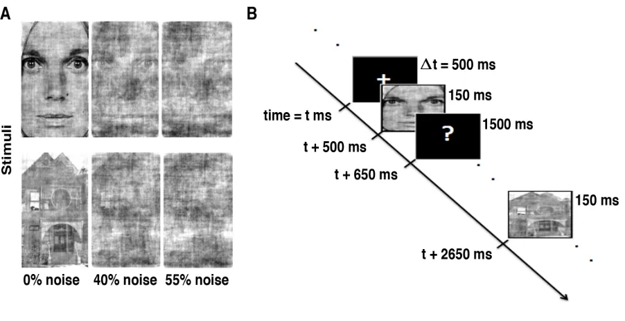
3.2.2 Stimuli

We used a total of twenty-eight images of faces and houses (14 images of each category).

Face images were from the Ekman series (124). Fast Fourier transforms (FFT) of these images

were computed, providing twenty-eight magnitude and twenty-eight phase matrices. The average

magnitude matrix of this set was stored. Stimulus-images were produced from the inverse FFT

(IFFT) of average magnitude matrix and individual phase matrices. The phase matrix used for

the IFFT was a linear combination of the original phase matrix computed during the forward

Fourier transforms and a random Gaussian noise matrix. The resulting images all had an

identical frequency power spectrum (corresponding to the average magnitude matrix) with

graded amounts of noise as done in previous studies (1, 47, 125). Finally, the stimuli consisted of

three different noise-levels: 0%, 40% and 55% (i.e., clear stimuli, 40% noisy stimuli, and 55%

noisy stimuli). The E-Prime 2.0 software was used to display the stimuli and control the task

sequences.

3.2.3 Experimental design

Prior to the experimental task, the participants were briefly explained about the task

paradigm. Participant sat in a dark room (the only source of light was from the experimenter’s

computer screen) and viewing distance was ~60 cm (chin rest). Figure 3.1 shows a schematic of

experimental paradigm used. The experiment consisted of 4 blocks of 168 trials (672 trials in

total with 224 trials for each noise level). On each trial, a small fixation cross (‘+’ in the middle

of the screen) was presented for 500 ms. Then a stimulus was presented for 150 ms, followed by

a black screen with a question mark (‘?’) for 1500 ms, during which time participants were

allowed to indicate their decision (either face or house) by a keyboard button press. Responses

Figure 3.1 Experimental design.

A) Stimuli with three noise-levels, B) task paradigm: stimuli were presented for 150 ms, followed by black screen with question mark (‘?’) for 1500 ms during which time participants responded with a keyboard button press.

3.2.4 Data acquisition and preprocessing

EEG data were acquired with a 64-channel EEG system from Brain Vision LLC

(http://www.brainvision.com). The analog signal was digitized at 500 Hz. The impedances of

each electrode were kept below 10 kΩ, and the participants were asked to minimize blinking,

head movements, and swallowing. EEG data were band-pass filtered between 1 and 100 Hz, and

notch filtered to remove 60 Hz AC-line noises. The eyes blinking were removed using

independent component analysis (ICA)-based ocular correction. Data from bad electrodes were

discarded and replaced, when appropriate, by spatial interpolation from the neighboring working

electrodes. These preprocessing steps were done using Brain Vision Analyzer 2.0

3.2.5 Data Analysis

The preprocessed EEG data were analyzed in the following main steps:

3.2.5.1 Computation of ERPs

Continuous EEG data were segmented into trials of 400 ms duration (post-stimulus: 0 to

400 ms) based on the stimulus onset times as a reference. The trials that had three standard

deviations below or above the global mean across time in each subject were considered as

outliers (126) and they were discarded from the subsequent analysis.

3.2.5.2 EEG-source and single-trials source waveforms reconstruction

All correct trials (ERPs of correct percept) from all three noise conditions were grand

averaged and imported to BESA software version 5.3.7 (www.besa.de) to reconstruct EEG

sources. We used the low resolution electromagnetic tomography (LORETA) (127), which is

also referred as Laplacian weighted minimum norm, to reconstruct the EEG sources. LORETA is

an extensively used source localization technique in EEG studies for both cortical and deep brain

structures (10, 122, 128-130), including insula and hippocampus (10, 129, 130). Depth weighting

strategy implemented in LORETA overcomes the problem of surface-restricted localization

methods, such as minimum norm estimates (MNE) (131-133). LORETA uses the Talairach

atlas coordinates of Montreal Neurological Institute (MNI) MRI average of 305 brains

and computes the inverse solution at 2394 voxels with spatial resolutions of 7 mm

(131, 134). It is based on the assumption that the smoothest of all possible neural activity

distributions is the most plausible one. This assumption is also supported by electrophysiology,

where neighboring neuronal populations show highly correlated activity while EEG-LORETA

results are the activity rendered by neighboring voxels with maximally similar activity (122, 132,

perpendicular to the local cortical surface based on neurophysiological information that the

sources of EEG are postsynaptic currents in cortical pyramidal cell, and that the direction of

these currents is perpendicular to the cortical surface (136, 137). Peak activities of these sources

were marked as the network nodes for connectivity analyses. Using single-trials EEG data, we

fitted dipoles at the locations of peak activation of localized sources of SN—the rAI, lAI, and

dACC based on our hypothesis—with dipole orientation presented in Table 1. Similarly, we

also fitted dipoles at the location of peak activation of localized sources of VTC-DLPFC

network: that is, at the FFA, PPA, and DLPFC (Table 2). The single-trials source signals were

then extracted using a four-shell spherical head model and a regularization constant of 1% for the

inverse operator. These source signals were used for the connectivity analyses.

3.2.5.3 Power and Granger causality spectral analyses

The power spectra can be computed using parametric and nonparametric approaches (4,

40, 41). To find the proper model order (which was four), we compared the spectral power from

both parametric and nonparametric approaches at different model orders and picked the model

order that rendered the lowest power difference between two approaches.

As the SN nodes showed a dominant activation at ~75-140 ms (as shown in Table 1), we

tried to cover dominant activation time frame in a single time frame while computing the power

and GC spectra at different time windows. We calculated the power and GC spectra from source

waveforms of SN nodes in four consecutive time frames: 0-75 ms, 75-150 ms, 150-225 ms, and

225-300 ms to uncover how the nodes and network activity changes with time. Besides time

frame wise GC calculations, we also computed GC spectra using a sliding window technique

(138, 139) by selecting a window size of 50 ms and sliding it every 2 ms to further observe how

computed from surrogate data (that is, from SN nodes) by using permutation tests and a

gamma-function fit (120, 140) under a null hypothesis of no interdependence at the significance level p <

10-4. The causal outflow at a node (See Eq. 1.2) is computed as the total GC flowing out from a

node minus total GC flowing in to that node in beta band (13-30 Hz).

For VTC-DLPFC network, as the FFA, PPA, and DLPFC showed dominant activation at

~130-240 ms (as shown in Table 2), we tried to cover dominant activation time frame of those

nodes in a single time frame while computing the power and GC spectra at different time

windows. We calculated the power and GC spectra from source waveforms of FFA, PPA, and

DLPFC in three consecutive time frames: 0-125 ms, 125-250 ms, and 250-375 ms to uncover

how the nodes and network activity changes with time. Besides time frame wise GC calculations,

we also computed GC spectra using a sliding window (138, 139) to further examine how GC

patterns change over time. The threshold value of GC, for statistical significance, was computed

from surrogate data (that is, from FFA, PPA, and DLPFC) by using permutation tests and a

gamma-function fit (120, 140) under a null hypothesis of no interdependence at the significance

level p < 10-3. The causal outflow at a node (See Eq. 1.2) is computed as the total GC flowing

out from a node minus total GC flowing in to that node in beta band (13-30 Hz) and gamma

(30-100 Hz), respectively.

3.2.6 Brain-behavioral correlation.

The response time (RT) of each participant for each stimulus was recorded. To see the

brain-behavioral correlation with the increase in noise level in stimuli, RTs were converted into

z-scores and plotted with GC. The relationship between GC and RT was tested using both

Spearman’s rank correlation and Pearson’s correlation. If p < 0.05 for both, the correlation was

3.3 Results

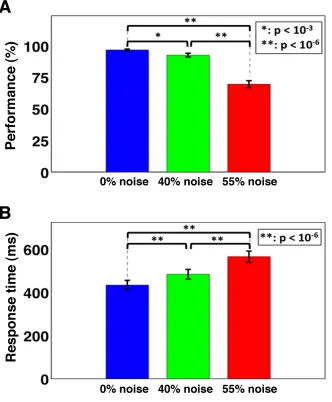
3.3.1 Behavioral results

The mean performance percent—a ratio of the number of correct responses to the total

number of responses multiplied by 100 and averaged over all participants—was highest for

stimuli with 0% noise level (mean: 96.80%, standard deviation: 0.71%) compared to the stimuli

with 40% noise level (mean: 92.68%, standard deviation: 1.54%) and 55% noise level (mean:

69.67%, standard deviation: 2.74%). Repeated measures analysis of variance (RMANOVA)

(141) showed the significant effect of noise levels (task difficulty) on the performance (F(2,44) =

150.43, p = 0.000003) and the response time (RT) (F(2,44) = 132.74, p = 0.000000). Pair t-test

post hoc analyses followed by false discovery rate (FDR) multiple comparisons (142) further

revealed that performance significantly decreased with the increase in noise level (p < 10-3;

FDR-corrected). The mean RT—the time taken to indicate the decision by pressing a keyboard button

press and averaged over all participants—was shorter for stimuli with 0% noise level (mean:

434.02 ms, standard deviation: 22.09 ms) compared to the stimuli with 40% noise level (mean:

484.28 ms, standard deviation: 22.66 ms) and 55% noise level (mean: 565.70 ms, standard

deviation: 25.73 ms). Pair t-test post hoc analyses followed by FDR multiple comparisons further

illustrated that the RT significantly increased with the increase in noise level (p < 10-6;

Figure 3.2 Behavioral responses for all three noise-levels.

A) Behavioral accuracy (performance %) significantly decreased, but B) the response

time significantly increased with an elevated noise in the stimuli.

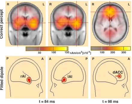
3.3.2 Brain results

3.3.2.1 Salience network dynamics

The average ERPs for correct decisions were used to compute localized sources

(inverse solutions) in LORETA (127). Figure 3.3 shows the locations of the peak source

fitted dipoles in the SN nodes (second row) to obtain the single-trials source

waveforms.

Figure 3.3 Spatiotemporal profiles of peak source-level brain activity over the SN nodes.

The first row shows peak source-level brain activity over the rAI and the lAI at 84 ms, and the dACC at 98 ms, and the second row shows the fitted dipoles on those nodes.

The earliest peak activation occurred in the visual area (BA17/18: V1/V2) at ~60

ms. The activation in the SN nodes started at ~76 ms after the stimulus onset.

Maximum peak activations occurred at ~84 ms in the rAI and lAI (BA47/13),

locations, dipole orientations of SN nodes in the source model, and dominant

activation time frames of cortical sources. The dipoles fitted at the locations and

orientations shown explained approximately 80% of the variance in the EEG signal for

trials with correct responses.

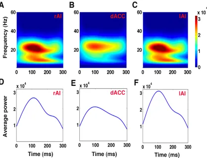
We computed power spectra using the wavelet technique (Figure 3.4) and GC

spectra using a sliding window (Figure 3.5) to see the activity over the entire time. To

further access how power and GC spectra change over time, we then performed

calculations at four time frames. Power spectra computed in four consecutive time

frames—TF1: 0 ms to 75 ms, TF2: 75 ms to 150 ms, TF3: 150 ms to 225 ms, and TF4: 225 ms

to 300 ms—at the rAI, lAI, and dACC showed peak activity in beta band when the

participants viewed clear stimuli (see Figure A.1).

Table 1 Anatomical location, dipole orientation, and dominant activation timeframe of the SN nodes.

Brain areas Talairach coordinates

x, y, z (mm) orientations Dipole

x, y, z

Dominant activation period

(ms)

Right anterior insula (rAI)

35.0, 9.0, -7.0 0.9, 0.3, -0.4 78 – 142

Left anterior

insula (lAI) -33.0, 11.0, -8.0 -0.9, 0.4, -0.3 76 – 144

Dorsal anterior cingulate cortex

(DACC)

Figure 3.4 Power spectra of the SN nodes as a function of time and frequency for stimuli with 0% noise.

The first row (panels A, B, C) shows wavelet power at the rAI, dACC, and lAI for clear stimuli (0% noise) with peak beta activity in around 75 ms to 150 ms compared to other time frames, and the second row (panels D, E, F) represents the average power (averaged over beta band) showing peak activity at ~100 ms in the rAI, dACC, and lAI.

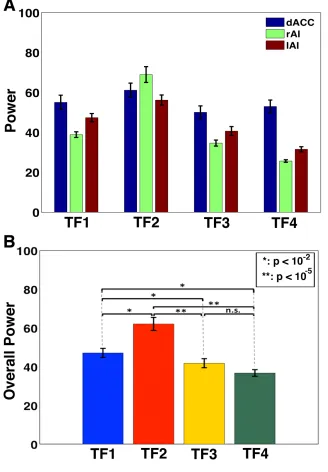
Figure 3.6 shows power comparison of nodes of the SN among TF1, TF2, TF3 and

TF4. Overall power over the SN nodes in TF2 is significantly higher compared to other

TFs. GC spectra were computed to assess the oscillatory network interactions among

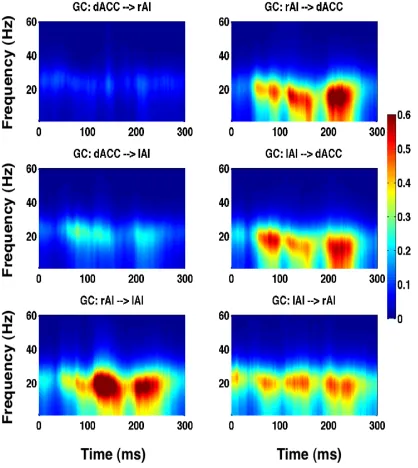
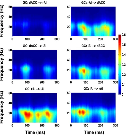
Figure 3.5 Granger causality spectra among the SN nodes as a function of time and frequency for stimuli with 0% noise.

Granger causality (GC) spectra as a function of entire time window (sliding time in milliseconds) and frequency for stimuli with 0% noise-level illustrating beta band activity. The first row shows GC between dACC-rAI pair, second row shows GC between dACC-lAI pair, and third row displays GC between rAI-lAI pair.

Figure 3.6 Power comparison of the SN nodes among four consecutive time frames for stimuli with 0% noise.

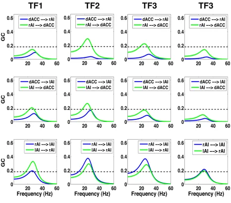
Figure 3.7 presents GC spectra as a function of frequency, where horizontal lines

represent statistically significant threshold value. Beta band network interactions

between the SN nodes are enhanced in the TF2 (second column) compared to the rest

of the TFs (other columns).

Figure 3.7 Granger causality spectra between all possible pairs of the SN nodes at four consecutive time frames for stimuli with 0% noise.

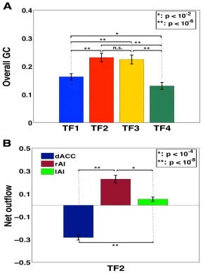
The overall connectivity strength of TF2 and TF3 were significantly higher than

those of others, with the biggest strength in TF2 (Figure 3.8A). Causal outflow

calculations in TF2 (the time frame of biggest overall connectivity strength) further

showed the rAI as a main ‘cortical outflow hub’ and the dACC as a main ‘cortical

inflow hub’ within the SN (Figure 3.8B).

Figure 3.8 Comparison of overall Granger causality and calculation of net outflow for stimuli with 0% noise.

time frame of highest connectivity strength (TF2) showed the rAI as a main outflow hub (p indicates statistically significant difference).

Power spectra were also computed for TF1, TF2, TF3, and TF4 at the rAI, lAI,

and dACC when participants viewed the stimuli with 40% and 55% noise-levels (see

Figures A.2, A.4). Power spectra calculations also showed peak activity in the beta

band. GC spectra were calculated to see the oscillatory network interactions among the

SN nodes in the entire time window (Figure 3.9 and Figure 3.10). GC spectra were

computed at four time frames to better assess the time dependence of the oscillatory

network interactions among the SN nodes.

Beta band network interactions among the SN nodes were suppressed for noisy

stimuli compared to clear stimuli in the TF2 (see second columns of Figures 3.7, A.3,

A.5). Overall causal interactions among the SN nodes were further compared between

noise-levels by paired t-tests to assess the significant effect of task difficulty. We found that the overall

information flow was significantly suppressed when the noise-level was elevated from 0% to

40%. Overall causal interactions were further significantly suppressed in the SN when the

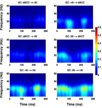
Figure 3.9 Granger causality spectra among the SN nodes as a function of time and frequency for stimuli with 40% noise.

Figure 3.10 Granger causality spectra among the SN nodes as a function of time and frequency for stimuli with 55% noise.

Figure 3.11 Comparison of Granger causality strengths among noise levels.

Granger causality (GC) connectivity strengths among SN nodes among all three noise-levels in the TF2: 75-150 ms. Overall connectivity strength is significantly suppressed with an elevated noise in the stimuli (p indicates statistically significant difference).

The difficulty levels—expressed in terms of behavior response times—were found to be

significant and negatively correlated with the measures of network activity for all possible

connections between cortical areas of the SN, except for the dACC to lAI flow, in the TF2

(75-150 ms). The correlation coefficient (r) and the corresponding p-value of all possible connections

Figure 3.12 Relation between Granger causality and response time.

Granger causality (GC) decreased with difficulty level of tasks, expressed in terms of response time of all three noise-levels, in TF2: 75-150 ms (r represents correlation coefficient and p < 0.05 represents statistically significant correlation).

3.3.2.2 VTC-DLPFC network dynamics

The average ERPs for correct responses were computed for clear stimuli (faces and

houses, separately) to examine the related ERP features over occipital-temporal channels. Figure

3.13A is Brain Products 10-20 EEG system showing standard channel information. We found

first negative peak at ~170 ms so called N170-component. The N170-component of ERPs over

and PO7) showed relatively right and left lateralized activity for clear faces and clear houses,

respectively. Moreover, ERPs for clear faces are relatively higher than that of houses.

Figure 3.13 Event related potentials over the occipital-temporal channels.

The average ERPs for correct responses were used for the inverse technique,

LORETA (127), to find the cortically localized sources. Figure 3.14 shows the location

of peak source activity (shown by crossing of lines) as it traversed the cortical surface

(first row), and the locations and orientations of fitted dipoles used to obtain the

single-trials source waveforms (second row). The earliest peak of cortical activity occurred in

the visual area (BA17/18) at ~60 ms after stimulus onset. We observed activation in

the areas of ventral temporal cortex (BA37: the right FFA and the left PPA) at ~160 ms, and

finally in the left DLPFC (BA9) at ~224 ms. Table 2 lists the ERP source locations, dipole

orientations of the source model, and dominant activation time frame of cortical sources.

The dipoles fitted at the locations and orientations shown explained approximately

80% of the variance in the EEG signal for trials with correct responses.

Figure 3.14 Spatiotemporal profiles of activity over the VTC-DLPFC nodes.

We computed GC spectra using a sliding window (Figure 3.15) to see the

activity over the entire time. To further access how power and GC spectra changes over

time, we then performed calculations at three timeframes.Power spectra computed in

the three consecutive time frames—TF1 (0-125 ms), TF2 (125-250 ms), and TF3

(250-375 ms)—at the DLPFC, FFA and PPA showed peak activity in the beta band and

gamma band when the participants perceived clear stimuli (0% noisy stimuli). Figure

3.16 shows the power computed at these nodes in the TF1, TF2 and TF3. Overall power over

these nodes was compared among these TFs using paired t-test. We found that beta

power was significantly higher in TF2 compared to other TFs, however gamma power

was significantly higher in TF1. GC spectra were calculated to assess the oscillatory

neural network interactions among these nodes.

Table 2 Anatomical location, dipole orientation, and dominant activation timeframe of the VTC-DLPFC nodes.

Brain areas Talairach coordinates

x, y, z (mm) orientations Dipole x, y, z

Dominant activation

period (ms)

Right fusiform face area (R FFA)

36.0, -47.0, -16.0 0.6, -0.7, -0.4 140 – 190

Left parahippocampal place area ( L PPA)

-30.0, -45.0, -10.0 -0.5, -0.8, -0.3 145 – 200

Left dorsolateral prefrontal cortex

(DLPFC)

Figure 3.15 Granger causality spectra among the VTC-DLPFC nodes as a function of time and frequency for stimuli with 0% noise.

Figure 3.16 Power comparison at the VTC-DLPFC nodes among three consecutive time frames for stimuli with 0% noise.

Figure 3.17 Granger causality spectra among the VTC-DLPFC nodes in three consecutive time frames for stimuli with 0% noise.

Figure 3.18 Comparison of overall Granger causality among three consecutive time frames and calculation of net outflow for stimuli with 0% noise.

Figure 3.17 shows GC spectra as a function of frequency, where horizontal lines

represent statistically significant threshold value. Beta band network interactions

among these nodes are enhanced in TF2 relative to the other TFs (other columns). The

overall connectivity strength between these nodes was significantly higher in TF2

compared to other TFs (Figure 3.18A). Net outflow calculations at each node in TF2

(time frame of highest activity in terms of power and connectivity) showed that the

FFA and PPA as the main outflow hubs and the DLPFC as a main inflow hub in the

network (Figure 3.18B). In the gamma band, network interactions were enhanced in

TF1 over the other TFs (other columns). The overall connectivity strength among these

nodes was significantly higher in TF1 compared to other TFs (Figure 3.18C). Net

outflow calculations at each node in TF1 (time frame of highest activity in terms of

power and connectivity) showed the DLPFC as a main outflow hub in the network

(Figure 3.18D).

Power spectra were also computed in TF1, TF2 and TF3 at the DLPFC, FFA

and PPA when participants perceived the stimuli with 40% and 55% noise-levels.

Power spectra calculations also showed peak activity in beta band and gamma band.

Both beta and gamma overall powers were significantly enhanced with task-difficulty

in their respective highest activity timeframe (Figure 3.19). GC spectra were computed

Figure 3.19 Power comparison at the VTC-DLPFC nodes among all three-noise levels.

Figure 3.20 Granger causality spectra among the VTC-DLPFC nodes as a function of time and frequency for stimuli with 40% noise.

Figure 3.21 Granger causality spectra among the VTC-DLPFC nodes as a function of time and frequency for stimuli with 55% noise.

Figure 3.22 Comparison of Granger causality strengths among the VTC-DLPFC nodes among all three-noise levels.

Comparison of Granger causality (GC) connectivity strengths among the FFA, PPA, and DLPFC among all three noise levels: in the TF2 (125-250 ms) for beta band (A, B), and in the TF1 (0-125ms) for gamma band (C, D).

We computed GC spectra using a sliding window (Figure 3.20 and Figure 3.21)

GC spectra change over time, we then performed calculations at three time frames. Beta

overall network interactions among these nodes were compared between the three noise-levels in

TF2 by paired t-test to assess the significant effect of task difficulty. We found that beta overall

information flow was significantly suppressed when the noise-level was elevated from 0% to

40%. Overall causal interactions among these nodes were further showed decreasing patterns

when the noise-level was elevated from 40% to 55% (Figure 3.22). One the other hand, gamma

overall information flow showed increasing patterns, specifically a more enhanced feature

between the FFA and the PPA (Figure 3.22 C), with the increase in noise level of the stimuli in

TF1.

In beta band, we uncovered that the response time (or the difficulty level) was negatively

correlated with the measures of network activity for all possible connections between the

DLPFC, FFA and PPA in TF2. In gamma band, the response time (or the difficulty level) was

positively correlated with the measures of network activity, especially in the FFA-PPA pair, in

TF1. The correlation coefficient (r) and the corresponding p-value of all possible connections

Figure 3.23 Relation between Granger causality and response time in beta band.

Figure 3.24 Relation between Granger causality and response time in gamma band.

Granger causality (GC) increased with difficulty level of tasks (expressed in terms of response time for all three noise-levels), especially in FFA-PPA pair (E, F), in TF1: 0-125 ms in gamma band (r represents correlation coefficient and p < 0.05 represents statistically significant correlation).

3.4 Discussion

3.4.1 Salience network dynamics

Behaviorally important events are responsible to activate the SN (67, 68). The AI and

dACC are among the most frequently activated brain areas in a wide range of functional

(66, 144, 147-149). As the SN nodes—the rAI, lAI and dACC—are often co-activated in fMRI

BOLD responses (69, 150) it is therefore difficult to clearly identify their distinct functional roles

within a network. In this study, using EEG recordings and perceptual decision-related

reconstructed EEG sources, we looked at the temporal changes of network activity flow within

SN. Using spectral GC analyses, we found that beta oscillation bound these nodes in the SN. The

beta power and beta causal interactions were significantly higher at the nodes and network in the

time frame 75-150 ms compared to other time frames. The analysis of the net beta causal outflow

(out – in causality) patterns showed that the rAI acted as a main cortical outflow hub of the SN

consistent with previous fMRI studies of the SN (69, 90). We also found that the beta causal

interactions within the SN were significantly suppressed with the task difficulty (noise level).

The causal outflow was negatively correlated with the response time.

We found that the key nodes of SN—the rAI, lAI and dACC—activated at around 100

ms after stimulus onset. These brain regions have been demonstrated as also being activated for a

variety of tasks in previous fMRI investigations (67-69). Electrophysiological recordings

combined with source localization techniques (113, 151) reported that the dACC responds to

salient events, such as error detection, in the time frame of 80-110 ms. The timing of dominant

activation of the dACC in our study was consistent with those studies. Similarly, the AI was

reported as being activated at ~60 ms after stimulus onset, however it was in a thermo-sensory

domain (152). Previous study on monkeys had found that the AI activated at ~65 ms after

stimulus onset, however it was in an auditory domain (153). Timings of activations demonstrated

in our study were not only close in line with previous studies that considered either AI or dACC,

but also resolved the overall time frame of activations that appeared in rAI, lAI and dACC.