Improving real time inflow forecasting into hydropower reservoirs through a complementary modelling framework

www.hydrol-earth-syst-sci.net/19/3695/2015/ doi:10.5194/hess-19-3695-2015

© Author(s) 2015. CC Attribution 3.0 License.

Improving real-time inflow forecasting into hydropower reservoirs

through a complementary modelling framework

A. S. Gragne1, A. Sharma2, R. Mehrotra2, and K. Alfredsen1

1_{Department of Hydraulic and Environmental Engineering, Norwegian University of Science and Technology,} Trondheim, Norway

2_{School of Civil and Environmental Engineering, The University of New South Wales, Sydney, Australia} Correspondence to: A. S. Gragne ([email protected])

Received: 12 October 2014 – Published in Hydrol. Earth Syst. Sci. Discuss.: 30 October 2014 Revised: 13 August 2015 – Accepted: 14 August 2015 – Published: 27 August 2015

Abstract. Accuracy of reservoir inflow forecasts is in-strumental for maximizing the value of water resources and benefits gained through hydropower generation. Im-proving hourly reservoir inflow forecasts over a 24 h lead time is considered within the day-ahead (Elspot) market of the Nordic exchange market. A complementary modelling framework presents an approach for improving real-time forecasting without needing to modify the pre-existing fore-casting model, but instead formulating an independent addi-tive or complementary model that captures the structure the existing operational model may be missing. We present here the application of this principle for issuing improved hourly inflow forecasts into hydropower reservoirs over extended lead times, and the parameter estimation procedure refor-mulated to deal with bias, persistence and heteroscedasticity. The procedure presented comprises an error model added on top of an unalterable constant parameter conceptual model. This procedure is applied in the 207 km2 Krinsvatn catch-ment in central Norway. The structure of the error model is established based on attributes of the residual time series from the conceptual model. Besides improving forecast skills of operational models, the approach estimates the uncertainty in the complementary model structure and produces proba-bilistic inflow forecasts that entrain suitable information for reducing uncertainty in the decision-making processes in hy-dropower systems operation. Deterministic and probabilis-tic evaluations revealed an overall significant improvement in forecast accuracy for lead times up to 17 h. Evaluation of the percentage of observations bracketed in the forecasted

95 % confidence interval indicated that the degree of success in containing 95 % of the observations varies across seasons and hydrologic years.

1 Introduction

Hydrologic models can deliver information useful for man-agement of natural resources and natural hazards (Beven, 2009). They are important components of hydropower plan-ning and operation schemes where it is essential to estimate future reservoir inflows and quantify the water available for power production on a daily basis. The identification and rep-resentation of the significant responses of hydrologic systems have been diverse among hydrologists. Different hydrolo-gists have incorporated their perceptions of the functioning of hydrologic systems into their models and come up with several rival models; some of them process based and oth-ers data based (for thorough reviews of the historic devel-opment of hydrologic modelling refer to Todini, 2007 and Beven, 2012). These models can be grouped into two main classes, conceptual and data-driven models.

hy-Solomatine and Shrestha, 2009).

Usefulness of a model for operational prediction is deter-mined by the level of accuracy to which the model repro-duces observed hydrologic behaviour of the study area. In operational applications, evaluation of how well the models capture rainfall–runoff processes, especially the snow accu-mulation and melting process in cold regions, is important because of the extent to which the models accurately repro-duce the reservoir inflows can significantly influence the ef-ficiency of the hydropower reservoir operation and subse-quently the power price. Application of hydrologic models for reproducing historic records can suffer from inadequacy in model structure, incorrect model parameters, or erroneous data. Consequently, despite failing to reproduce the observed hydrographs exactly, they enable simulation of hydrologic characteristics of a study catchment to a fair degree of ac-curacy. It gets more challenging when using the models in the operational set-up for forecasting the unknown future just based on the known past, which the model might not cap-ture accurately. In the context of the Norwegian hydropower systems, being unable to predict future reservoir inflows ac-curately has negative consequences on the power producers. Norway’s energy producers have to pledge the amount of en-ergy they produce for next 24 h in the day-ahead market and if unable to provide the pledged amount of energy the chance of incurring losses is very high. Estimation of future reser-voir inflows (be it long- or short-term) involves estimating the actual (initial) state of the basin, forecasting the basin inputs during the lead time, and describing the water move-ment during the lead time (Moll, 1983). Hence, the quality of a hydrologic forecast depends on the accuracy achieved and methodology selected in implementing each of these aspects. In this study, we intend to use conceptual and data-driven models complementarily. A conceptual model with cali-brated model parameters is used as the fundamental model that approximately captures dominant hydrologic processes and forecasts the behaviour of the catchment deterministi-cally. A data-driven model is then formulated on the residu-als, the difference between observations and predictions from the conceptual model. By studying the whole set of residu-als and exploring the information they contain, important in-formation that describes the inadequacies of the conceptual model can be extracted. In general, this kind of information can be used for improving either the conceptual model it-self or the prediction skill of a forecasting system. Emulating the practice in most Norwegian hydropower reservoir

opera-model to capture all the physical processes exactly. Thus, in the operational sense, the data-driven models can play a com-plementary role by adjusting output of the conceptual model whenever the conceptual model needs corrective adaptation (e.g. Serban and Askew, 1991; World Meteorological Orga-nization, 1992).

Several example applications can be found in the scientific literature on using conceptual and data-driven models com-plementarily. For instance, Toth et al. (1999) compared per-formance improvements six autoregressive integrated mov-ing average (ARIMA)-based error models brought to stream-flow forecasts from a conceptual model to identify the best error model and data requirements. Shamseldin and O’Connor (2001) coupled a multi-layer neural network model on top of a conceptual rainfall–runoff model to im-prove accuracy of streamflow forecasts without interfering with the operation of the conceptual model. Similarly, Mad-sen and Skotner (2005) developed a procedure for improving operational flood forecasts by combining error models (lin-ear and non-lin(lin-ear) and a general filtering technique. Xiong and O’Connor (2002) investigated performance of four error-forecast models, namely, the single autoregressive, the au-toregressive threshold, the fuzzy auau-toregressive threshold and the artificial neural network updating models, for im-proving real-time flow forecasts and compared their results. Likewise, Goswami et al. (2005) examined the forecasting skill of eight error-modelling-based updating methods. A re-cent review on the application of error models and other data assimilation approaches for updating flow forecasts from conceptual models can be found in Liu et al. (2012).

As reviewed above, the principle of complementing con-ceptual models with data-driven models has enjoyed appli-cations in real-time hydrologic forecasting since the 1990s. The methodological contribution of the present work is refor-mulation of the parameter estimation procedure for the data-based model. We recognize that the bias, persistence and heteroscedasticity seen in the residuals from the conceptual model reflect structural inadequacy of the conceptual model to capture the catchment processes and, hence, are important in defining the manner the residual series is dealt with. Ac-cordingly, we describe the reservoir inflows in a transformed space and present an iterative algorithm for estimating rameters of the data-driven model and the transformation pa-rameters jointly.

same concept of complementing conceptual models with data-driven models. First, it attempts to provide hourly reser-voir inflows of improved accuracy 24 h ahead. The earlier papers mainly succeeded in improving forecasts for forecast lead times up to six time steps or incorporated a scheme to update the forecast system at an interval of six time steps. Second, an attempt is made in what follows, to produce a probabilistic forecast by estimating the uncertainty of the er-ror model, rather than only the deterministic estimate. This, thereby, enables forecast of an ensemble of reservoir in-flows, thereby allowing for a risk-based paradigm for hy-dropower generation to be put to use. Reasons as to why hydrologic forecasts should be probabilistic and the poten-tial benefits therein are presented and explained in Krzyszto-fowicz (2001). KrzysztoKrzyszto-fowicz (1999) described a method-ology for probabilistic forecasting via a deterministic hydro-logic model. Li et al. (2013) presented a review of scien-tific papers that provide various regression and probabilistic approaches for assessing performance of hydrologic mod-els during calibration and uncertainty assessment. Smith et al. (2012) demonstrate a good example of producing proba-bilistic forecasts based on deterministic forecast outputs. In this paper, the improvement levels achieved are evaluated deterministically using the same or similar metrics as past studies, and probabilistically using (i) the containing ratio (Xiong et al., 2009), which is also referred to as reliability score (e.g. Renard et al., 2010) and (ii) the probability in-tegral transform (PIT) plot. The technique is similar to the predictive Q–Q plot (e.g. Thyer et al., 2009) but assesses, in terms of the percentiles, how close a continuous random variable transformed by its own cumulative distribution func-tion (cdf) is to a uniform distribufunc-tion. We emphasise here that taking into account uncertainties emanating from vari-ous recognized sources and describing the degree of reliabil-ity of the inflow forecasts has important benefits. According to Montanari and Brath (2004), the Bayesian forecasting sys-tem (BFS) and the generalized likelihood uncertainty estima-tion (GLUE) are the popular methods for inferring the uncer-tainty in hydrologic modelling. Yet, the scope of producing probabilistic inflow forecasts in this study is limited to at-taching a certain probability to the deterministic forecasts, which are common in the Norwegian hydropower industry, based on analysis of the statistical properties of the error se-ries from the conceptual model, and assessing its degree of reliability.

In the next section, the complementary model set-up is formulated and the performance evaluation criteria are pro-vided. An example application is presented in the subsequent section. This includes description of the study area and data used, findings from the evaluation of the complimentary set-up and its components during calibration and validation, and results of forecasting skill assessment using deterministic and reliability metrics. Finally, concluding remarks are pro-vided.

2 Methodology

2.1 The conceptual model set-up

The widely applied conceptual hydrologic model, HBV (Hydrologiska Byråns Vattenbalansavdelning) (Bergström, 1995), is used in this study. The version used allows for di-viding the study catchment up into 10 elevation zones. A deterministic HBV model with already calibrated model pa-rameter values was assumed to take the role of the opera-tional hydrologic models Norwegian hydropower companies commonly use for forecasting reservoir inflows. In the op-erational set-up, the air temperature and precipitation input over the forecast lead time are obtained from the Norwegian Meteorological Institute (http://www.met.no). As this study aims to improve hydrologic forecasts into the hydropower reservoirs by complementing the conceptual model by an er-ror model, we assume that the predictions from the HBV model are made using the best possible input data. Hence, the observed air temperature and precipitation data are used as input forecasts in hindcast.

2.2 The complementary error model

The error model aims at exploiting the bias, persistence and heteroscedasticity in the residuals and estimating the errors likely to occur in the forecast lead time. Forecasting the er-ror in the lead time is regarded as a two-step process: offline identification and estimation of the error model, and error predictions based on most recent information.

2.2.1 Identification of the model structure

An error model that captures the structures the processes model is missing should lead to a zero-mean homoscedas-tic residual series from the modelling framework. In order to identify the right structure and establish a parsimonious model that adequately describes the data, we diagnose the residuals and address the bias, persistence and heteroscedas-ticity the series might exhibit as follows.

First and foremost, we transform the observed (Q) and the predicted (q, from the conceptual model) inflows intoˆ zand

ˆ

z, respectively. This way we deal with the heteroscedasticity seen in the residuals by making repeated use of Eq. (1) with the appropriate inflow term.

ˆ

zt =

(

ˆ

qt+βλ−βλ−1 λ >0 log qˆt+β

λ=0, (1)

whereβandλare the transformation parameters.

popularity is deservedly right and further emphasize the ef-fectiveness of a very parsimonious model, such as the AR model, for error forecasting.

ˆ

et=

p

X

i=1

aiet−i, (2)

where p designates the length of the lag time, and a1, a2, . . . ,apare coefficients of the AR model.

In order to provide improved hourly reservoir inflow fore-casts over a 24 h lead time, the error-forecasting model takes the form of Eq. (3). In order to overcome lack of observed residuals encountered for forecast lead time (f) longer than one-step ahead, it is necessary to utilize estimated errors as inputs (see Eq. 3). The number of estimated error values to be used as inputs depends on the identified order of the AR model and can vary across the forecast lead times.

ˆ

e_t+f =         

       

p P i=1

aiet+f−i forf=1 f−1

P i=1

aieˆt+f−i+ p P i=f

aiet+f−i forf≥2 andp≥f p

P i=1

a_ieˆ_t+f−i forf≥2 andp < f (3)

In its complete form, the error-corrected reservoir inflow forecast (z0) from the complementary modelling framework can be given as

z0_t+f = ˆzt+f+ µe+ ˆet+f. (4)

2.2.2 Parameter estimation

Parameters of the AR model can be set to the correspond-ing Yule–Walker estimates ofa1,a2, . . . ,ap given the auto-correlation function of the error series fulfils a form of the linear difference equation. However, in practice, Eq. (2) can be treated as a linear regression and parameters can be esti-mated by least squares method as demonstrated by Xiong and O’Connor (2002). An iterative algorithm suggested in Beven et al. (2008) is adopted for estimating the model parameters, while optimizing transformation of the inflow data. Adoption of a methodology that amalgamates parameter estimation and Box–Cox (Box and Cox, 1964) inspired transformation of inflow is useful for taking into account the heteroscedastic residuals and obtaining a normally distributed residual series from the error model. The parameter and inflow transforma-tion steps with a little modificatransforma-tion from Beven et al. (2008) over the calibration period (1, . . . ,T) are as follows:

given observation time step (t) equals (µe+ ˆet). Thus, the observed (ε) and forecasted (ε) errors at a given ob-ˆ

servation time step (t) can be related as εt= ˆεt+ηt, whereηt is a random noise that describes the total un-certainty originating from various sources.

4. Adjust (β,λ) and repeat the optimization until the resid-uals of the error model appear homoscedastic. Theηt term (step 3) is assumed to be unimodal, symmetric and unbounded random variable with a zero expected mean and second moment given asσ2.

2.3 Performance evaluation

In addition to visual evaluation of the hydrographs, perfor-mance of the present procedure is robustly analysed using deterministic and reliability metrics. The root mean square error (RMSE), relative error (RE) and the Nash–Sutcliffe efficiency (NSE) (Nash and Sutcliffe, 1970) are employed to evaluate efficiency of the models during calibration and validation deterministically. Evaluations are made with re-spect to varying forecast lead times and season-wise as well. Among the three statistical performance criteria, the RE (Eq. 5) measures the relative error between the total observed and predicted inflow volume. For a good simulation the value of RE is expected to be close to zero. Quantifying the relative error (RE) of the simulations/forecasts is important because it indicates how the inaccuracies affect a hydropower com-pany’s ability to deliver the amount of energy it has pledged to provide to the energy market. Therefore, special attention is given to the less aggregate version of RE, which we refer to as percentage volume error (hereafter PVE) and describe as follows.

RE=

P _z

t− ˆzt

P_z

t

×100% (5)

treats overestimates and underestimates separately. The num-ber of times each of the six absolute PVE classes appeared in the set or subset of interest (i.e. hydrologic year or sea-sons) is constructed by keeping score of the PVE class into which each and every residual fell in. Then the fraction of time in which each PVE class occurred is divided into the total number of points in the given set/subset and is reported as a percentage. This is designated as a “PVE count”. Model performance assessment using PVE (during simulation and forecasting) mainly focuses on assessing the change in the number of incidences in each PVE set, which in other words means the change in PVE counts. The PVE count/change in PVE count, along with the above-mentioned deterministic statistical criteria, is used for evaluating the simulation and forecasting skill of the complementarily set-up system (con-ceptual model+error model). As a metric for measuring the relative improvement in forecasting skills, high PVE counts for the low PVE classes (e.g. ≤10 %) are considered desir-able quality. The justification is that the penalty a power pro-ducer incurs when failing to deliver the pledged amount of power would be lesser if its forecasting system makes errors of lower PVE classes more frequently.

Another useful metric used for assessing forecasting skill of the complementary set-up is through uncertainty analy-sis. An interval forecast (Chatfield, 2000) can be constructed by specifying an upper and lower limit between which the future reservoir inflow is expected to lie with a certain prob-ability (1−α). The prediction interval for the inflow forecast is estimated using the Linear Regression Variance Estima-tor (LRVE) described by Shrestha and Solomatine (2006). Xiong et al. (2009) outlined several indices that can serve for describing the properties of prediction bounds of particu-lar probability and for comparative study of prediction inter-vals resulting from different uncertainty assessment schemes. The indices characterise the prediction bound either by the percentage of observations it contains, its bandwidth, or its symmetry relative to the observation. Of all indices, accord-ing to Xiong et al. (2009), the containaccord-ing ratio (CR), which describes the percentage of observed inflows falling in the desired interval percentage, is the widely used metric for assessing reliability of probabilistic forecasts. We adopt the CR metric for describing the reliability of the forecasts with the desired interval percentage of 95 % (α=0.05). In addi-tion to the CR, we verify the probabilistic forecasts graph-ically using the less formal PIT uniform probability plot. The working procedure as well as detailed application ex-amples can be found in Laio and Tamea (2007) and Thyer et al. (2009). Among others, Pokhrel et al. (2013) and Wang et al. (2009) demonstrated viability of the “PIT uniform prob-ability plot” approach for checking uniformity (and inves-tigating the causes, in cases of deviations from uniformity) without binning the data subjectively.

3 Example application

3.1 Study area and data

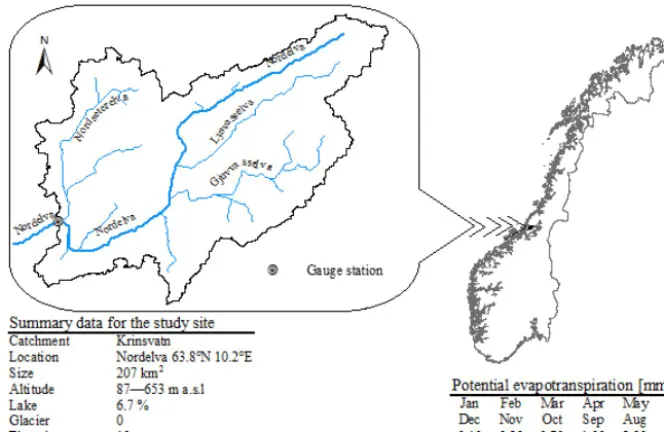
The Krinsvatn catchment is located in Nord Trøndelag County in mid-north Norway. It comprises an area of 207 km2 and about 57 % of the catchment is mountain area above the treeline. The elevation ranges from 87 to 628 m a.m.s.l. (above mean sea level) and is drained by the Stjørna/Nord River. The dominant land use is forest covering 20.2 % of the study site while marsh, lakes and farmlands cover about 9, 6.7 and 0.4 % of the catchment area, respec-tively. Figure 1 provides the location and main characteristics of the study site, and the daily potential evapotranspiration values used.

Observed hourly data of 11 water years (September 2000 to August 2011) were split into three sets used for warming-up (2000), calibrating (2001–2005) and validating (2006– 2010) the conceptual and the error models alike. Observed precipitation and temperature data of two meteorological sta-tions (i.e. Svar-Sliper and Mørre-Breivoll) in neighbouring catchments are used. Discharge data for the catchment are derived from water level records at the Krinsvatn gauge sta-tion. Romanowicz et al. (2006) outline the advantages to di-rect use of water-level information in hydrologic forecasting. Rating curve uncertainties and their influence on the accu-racy of flood predictions have been very well documented (e.g. Sikorska et al., 2013; Aronica et al., 2006; Pappenberger et al., 2006; Petersen-Overleir et al., 2009). Krinsvatn is con-sidered a stable discharge measurement site with few exter-nal influences, and the rating curve was updated in 2004. This study, however, considers the uncertainty of the rating curve to be one of the factors contributing to the total error expressed in Eq. (2) and does not address it separately.

3.2 HBV model for Krinsvatn catchment

The catchment is divided into 10 elevation zones in the HBV model set-up. Input data used are hourly areal precipitation, air temperature, and potential evapotranspiration. The model is run on an hourly time step for the water years 2000 to 2005 with the last 5 water years being used for model calibration. Calibration is carried out using the shuffled complex evolu-tion algorithm (Duan et al., 1993), with the NSE between the observed and predicted flows as an objective function. De-scription of the model parameters along the corresponding optimized values is provided in Table 1.

3.2.1 Overview of the conceptual model’s performance

simu-Figure 1. Location, characteristics and potential evapotranspiration estimates of the study catchment.

Table 1. Model parameters and corresponding optimized values.

Parameter Description Unit Optimized

value

Snow routine

TX Threshold temperature for rain/snow [◦C] 2.23

CX Degree-day factor for snowmelt (forest-free part) [mm day−1◦C] 9.95

CXF Degree-day factor for snowmelt (forested part) [mm day−1◦C] 5.21

TS Threshold for snowmelt/freeze (forest-free part) [◦C] 0.73

TSF Threshold for snowmelt/freeze (forested part) [◦C] −1.80

CFR Refreeze coefficient [mm day−1◦C] 0.04

LW Max relative portion liquid water in snow [−] 0.085

Soil and evaporation routine

FC Field capacity [mm] 306.87

FCDEL Minimum soil moisture filling for POE [−] 0.31

BETA Non-linearity in soil water retention [−] 3.84

INFMAX Infiltration capacity [mm h−1] 30.22

Groundwater and response routine

KUZ2 Outlet coefficient for quickest surface runoff [1/day] 1.65

KUZ1 Outlet coefficient for quick surface runoff [1/day] 0.99

KUZ Outlet coefficient for slow surface runoff [1/day] 0.42

KLZ Outlet coefficient for groundwater runoff [1/day] 0.09

PERC Constant percolation rate to groundwater storage [mm day−1] 1.60

UZ2 Threshold between quickest and quick surface runoff [mm] 122.34

UZ1 Threshold between quick and slow surface runoff [mm] 49.97

Table 2. Summary of overall and seasonal performance of the conceptual model during the calibration (September 2001 to Au-gust 2005) and validation (September 2006 to AuAu-gust 2011) peri-ods.

Seasons Calibration period Validation period

RMSE RE NSE RMSE RE NSE

[mm] [%] [−] [mm] [%] [−]

Overall 0.139 1 0.842 0.162 18.8 0.700 Autumn 0.147 1.8 0.724 0.147 11.3 0.769 Winter 0.182 −3.7 0.894 0.126 9.7 0.812 Spring 0.131 −2.7 0.709 0.246 24.6 0.509 Summer 0.073 28.2 0.641 0.079 38.2 0.592

lations match observations better during calibration than val-idation. High NSE values (>0.8) during both calibration and validation reveal that the inflow simulations fit the observed hydrographs best in the winter seasons. Nevertheless, it is ev-ident that model predictions in the validation period are prone to underestimation bias (RE>0). Season-wise assessment of the validation period reveals the conceptual model’s ten-dency to underestimate reservoir inflows in spring and sum-mer considerably. In light of what the NSE and RE metrics suggest, the lower RMSE values (i.e. for instance summer season) do not reflect superior model performances.

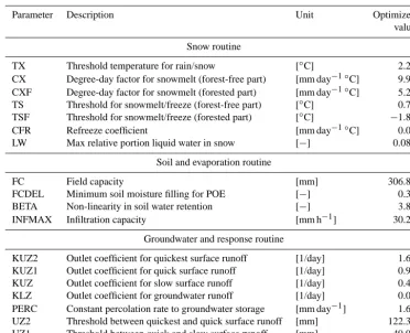
PVE counts of the six PVE classes (i.e.≤10, 10–20, 20– 30, 30–40, 40–50 and>50 %) are computed on the resid-uals between observed and simulated reservoir inflows. The stacked columns of Fig. 3a and b show how frequently each of the six absolute PVE classes occurred over the calibra-tion and validacalibra-tion period. The results reveal a large degree of discrepancy between observations and predictions during calibration and validation. Simulated inflows deviated from the corresponding observed values by a magnitude of more than±10 % in about 83.3 % (calibration) and 88.6 % (valida-tion) of the respective simulation time steps. Huge difference between observations and simulations is noted in the sum-mer season with absolute PVE of the class>50 % occurring in more than half of the simulation time steps throughout the calibration and validation periods. Winter simulations listed the highest level of occurrence of PVE of the class≤ ±10 % during both calibration and validation. Comparable to the re-sults in Table 2, volume errors in winter simulations do not seem to be a serious problem, probably because the season is predominantly a snow accumulation rather than runoff gener-ation period. Errors of the high absolute PVE classes scored high PVE counts in the spring and autumn seasons.

respec-Figure 3. Stacked-column plots of (1) PVE counts of the six absolute PVE classes (≤10, 10–20, 20–30, 30–40, 40–50 and>50 %) during calibration (a) and validation (b), and (2) the fraction of times under- and overestimation incidents corresponding to the six PVE classes occurred during calibration (c) and validation (d).

tively. In the validation period, the reservoir inflows are un-derestimated about 65.6 % of the time compared to overesti-mation in 33.4 % of the time. This is also revealed in the find-ings from statistical metrics in Table 2, which disclose the bias in the model. Yet, the results in Fig. 3 further reveal that the model predictions deviate from the observations at high discharges. For example, during the validation period 59.2 % of the time observations exceeded the predictions by mag-nitudes of more than 10 %. Such information is useful be-cause direct evaluation of observed and predicted values ex-plains the implications of model performance on the planning and operation of a hydropower system better than an aggre-gated variance-based statistic. From an operational manage-ment point of view, considerable underestimation of reser-voir inflows can have both short-term and long-term effects on the operation of a hydropower system. In the short-term, the company could be forced to release unvalued water espe-cially when the reservoir water level is close to its maximum capacity. Hence, the high percentage of underestimations that occur in the autumn and spring seasons (during calibration and validation) should not be tolerated because the inflows in the autumn and spring seasons are very important. On the one hand, substantial overestimation of reservoir inflows can at least expose any Norwegian hydropower company to unde-sirable expenses due to obligations to match the power sup-ply it has failed to deliver by dealing with other producers in the intra-day physical market (Elbas). Although overestima-tion does not seem to be a pertinent issue, Fig. 3d unmasks

that the inflows are overestimated by a magnitude>50 % at least 10 % of the time in all seasons.

3.2.2 Residual analysis

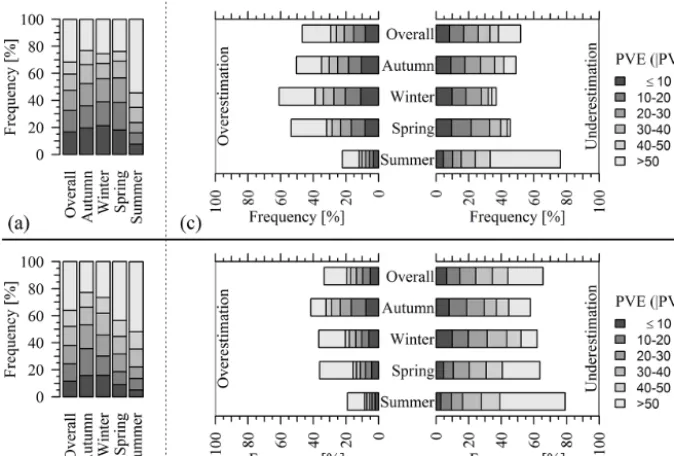
Following the example of Xu (2001), a Kolmogorov– Smirnov test is applied to residuals of the conceptual model. The test revealed that the residuals are not normally dis-tributed. The maximum deviation between the theoreti-cal and the sample lines is 0.130, which is larger than Kolmogorov–Smirnov test statistic of 0.008 at significance levelα=0.05.

Figure 4. Plots of (a) residuals from the conceptual model as a function of predicted inflow during the calibration period, (b) autocorrelation function of the residuals, and (c) partial autocorrelation functions of the residuals.

3mm are rare and occurred about 0.1 % of the time over the calibration and validation period.

Plots of autocorrelation and partial autocorrelation func-tions of the residual time series (Fig. 4b and c) indicate a strong time persistence structure in the error series. Rapid decaying of the partial autocorrelation function confirms the dominance of an autoregressive process, which the gradu-ally decaying pattern of the autocorrelation function also sug-gests. Thus, in order to obtain a Gaussian series, it is impor-tant to address issues of heteroscedasticity and serial correla-tion in the residual series. As the current study aims at utilis-ing the persistent structure in the residuals for supplementutilis-ing the forecasting system, the corrective action to be taken only aims at removing the heteroscedasticity. A successful way to do it is through transformation of the flow data (e.g. Enge-land et al., 2005). As outlined in the methodology section, the reservoir inflows (both observed and predicted) are trans-formed while estimating parameters of the error model.

3.3 Structure and performance of the error model

In accordance with the findings from the ACF and PACF plots discussed in Sect. 3.3.2, AR models of up to an or-der of p=3 were investigated while estimating parameters of the error model. As outlined in Sect. 2.2.2, coefficient of the AR(p) model and the transformation parameters were es-timated by minimizing the sum of the squares of the offsets

between the inflows (observed and predicted) in the trans-formed space, and assessment of whether the subsequent residuals from the complementary modelling framework ap-pear homoscedastic and exhibited correlation. The latter was assessed using the Kolmogorov–Smirnov (KS) statistic as a relative quantitative measure followed by visual inspection of the residual plots, which led to the selection of an AR(1) model with transformation parametersβ=41.4 andλ=0.9, bias correctionµe=0.021 and coefficienta1=0.97.

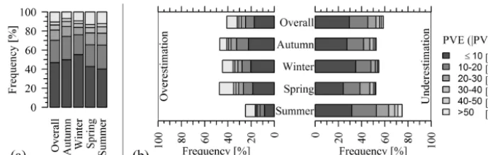
Figure 5. Stacked-column plots of (a) PVE counts of the six absolute PVE classes (≤10, 10–20, 20–30, 30–40, 40–50 and>50 %) observed in reservoir inflow forecasts from the complementary set-up, and (b) the corresponding fraction of times under- and overestimation incidents corresponding to the six PVE classes occurred. Hydrologic years 2006–2010.

that the residuals from the complementary forecasting sys-tem would be Gaussian is far from being true. As the aim of this study is to utilize the error and complementary models additively, we discuss in the next section the extent to which the complementary set-up boosted prediction ability in the forecasting mode and come back to the issue of violation of the Gaussian assumption in section 3.5, where we analyse the reliability of the forecasts probabilistically.

3.4 Forecasting skill of the complementary set-up

(deterministic assessment)

Imitating operational application of forecasting models in the Norwegian hydropower system, reservoir inflows for the day-ahead market (Elspot) are estimated using the presented forecasting system. The system has to run once a day at an hourly time step, sometime before 12:00 LT after retrieving the latest observations, and the inflow forecasts are issued for the next 24-hourly time steps beginning from 12:00 LT. Over-all performance of the complementary model in forecasting the reservoir inflows during the calibration and validation pe-riods is first discussed and is followed by evaluation of its forecasting skill with respect to forecast lead times. Evalua-tion of the forecast skill presented in this paper is based on assessment of forecasts made for the period between ber 2006 and August 2011 as the data sets from Septem-ber 2000 to August 2006 are used for calibrating the system.

3.4.1 Overall performance

Assessment of the overall forecasting skill of the comple-mentary set-up shows significant improvement in forecast ac-curacy. The RMSE and NSE statistical criteria computed be-tween forecasted and observed inflows are 0.095 and 0.896, respectively. RMSE values for the autumn, winter, spring and summer forecasts are 0.094, 0.090, 0.132 and 0.044, respec-tively, and the corresponding NSE values are 0.904, 0.905, 0.859 and 0.873.

Proving capability of the complementary set-up to reduce the bias revealed in the simulation forecasts from the

concep-tual model, which was pointed out in the previous section, the 24 h lead-time forecasts exhibited low-level underestimation bias with RE equal to 3.8 %. Degree of bias in the inflow fore-casts differed seasonally. The RE computed for each season in a decreasing order is summer (10.2 %), spring (4.6 %), au-tumn (2.9 %) and winter (0.7 %). The relatively higher bias in the spring and autumn forecasts can be related to runoff generation in the Krinsvatn catchment due to snowmelt or occurrence of precipitation in the form of rainfall, which can affect the persistence structure in the residual series obtained from the conceptual model.

Stacked-column plots in Fig. 5 display the occurrence level of each of the six PVE classes in the residual series between forecasts and observations. Visual comparison of stacked-column plots of Fig. 5 and Fig. 3 shows reduction in PVE count of the high PVE classes and increase in PVE counts of low PVE classes; e.g. PVE count for the PVE class>±50 % decreased by about 15 %, while PVE count for the PVE class≤ ±10 % grew by about 50 %. In order to assess this assertion, a further assessment is carried out by dividing the six PVE classes into two groups: low PVE (PVE≤ ±10 %) and high PVE (PVE>±10 %). Ratio be-tween seasonal PVE counts of the low and high PVE classes is taken and comparison is made on two sets of residual se-ries. These sets of residuals are (1) residuals from the sim-ulated forecasts (conceptual model) and (2) residuals from forecasts of the complementary set-up. Results are presented in Table 3. Apart from confirming the success in reducing PVE counts of high PVE errors, the results indicate that an equal level of success is not achieved in all four seasons. In relative terms, high PVE errors occur more often in the spring and summer forecasts. As pointed out earlier, this can be associated with the snowmelt and, to a certain degree, to rainfall incidents occurring in these seasons.

3.4.2 Forecast skill with respect to forecast-lead times

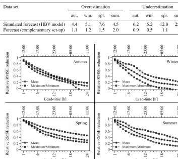
Table 3. Ratio between occurrence frequency of low PVE (≤10 %) and high PVE (>10 %) errors for the hydrologic years 2006–2010.

Data set Overestimation Underestimation

aut. win. spr. sum. aut. win. spr. sum.

Simulated forecast (HBV model) 4.4 5.1 7.6 4.5 6.2 5.2 12.8 25.4

Forecast (complementary set-up) 1.1 1.2 1.5 2.0 0.9 0.5 1.1 1.3

Figure 6. Summary of relative seasonal RMSE reductions as a function of forecast lead time (minimum, mean and maximum values com-puted from corresponding computations for the hydrologic years 2006–2010).

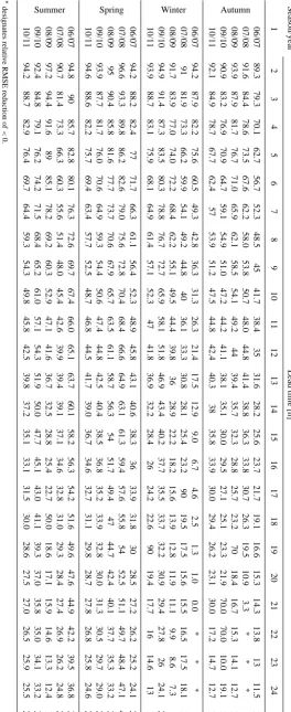
season of the hydrologic years between 2006 and 2010 are presented in Table 4. The results are also summarized in terms of the minimum, mean and maximum relative RMSE reduction as shown in Fig. 6. Excluding forecasts in autumn and winter seasons of the 2006 water year, relative RMSE reductions are observed in forecasts of short and long lead times. Of course, in all four seasons, the achieved level of improvement in forecast accuracy is high for short lead times and diminishes gradually with increased lead time. Results show that accuracy of the reservoir inflows in the spring and summer seasons are improved over the entire range of the forecast lead time. Likewise, reduction in RMSE is observed for all autumn and winter inflow forecasts except for the wa-ter years 2006 and 2007, respectively.

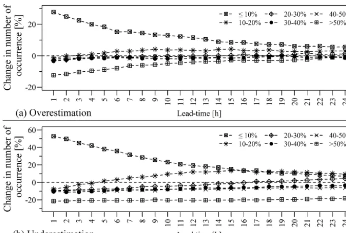
In order to get insight on the improvement level in a unit directly related to hydropower production, the change in PVE count of each PVE class is calculated. Change in PVE count of a given absolute PVE classes is the difference between the PVE counts for the complementary set-up and that for the conceptual model. The results are summarized as shown in Fig. 7. The figure shows that the PVE count of high mag-nitude absolute PVE classes are reduced and the opposite

Figure 7. Change in number of occurrence of the six absolute PVE classes (≤10, 10–20, 20–30, 30–40, 40–50 and>50 %) as a function of forecast lead time: (a) overestimation and (b) underestimation.

Calculation of the relative RMSE reduction and the change in PVE counts agree that the forecast accuracy is improved through the complementary set-up. The assessments further revealed that the degree of improvement weakens with in-creased forecast lead time. However, the relative RMSE re-duction computations indicate that in some occasions the simulated inflow forecasts stand out to be better. The relative RMSE reduction values for lead times longer than 20 h (Ta-ble 4) show that complementing the conceptual model with an error model is counterproductive in autumn and winter seasons of the water years 2007 and 2006, respectively.

3.5 Reliability of the inflow forecast

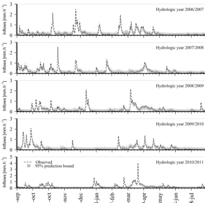
Computation of the CR for the entire forecast reveals that 95.8 % of the observations are inside the 95 % prediction in-terval. The inflow hydrographs (Fig. 8) confirm that most of the observed inflows are contained in the specified uncer-tainty bounds.

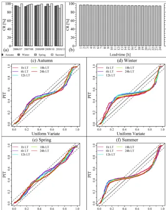
The percentage of observation points falling within the forecasted 95 % confidence interval varies from season to season and across hydrologic years (see Fig. 9a). All ob-served winter and summer inflows are bracketed in the 95 % uncertainty bound at least 95 % of the time. In general, the winter season is more of a snow accumulation period and a closer observation of the hydrographs (see Fig. 8) reveals that the summer hydrographs cover the recession and base flow portions of the annual hydrographs. Thus, better persis-tence structure and predictable discrepancies between sim-ulated forecasts from the conceptual model and the obser-vations. As Goswami et al. (2005) argued, the persistence

structure in residual series primarily arises from the dynamic storage effects of a catchment system.

accumula-Figure 8. Observed hydrograph (broken lines) and the forecasted 95 % confidence interval.

tion and melting processes can simply occur due to the er-ror in the input temperature record. Because of this, the per-sistence in the errors between simulated forecasts from the conceptual model and the observations can get weaker. Ac-cording to Goswami et al. (2005), some degree of persistence in the model input (i.e. rainfall) is another primary source of the persistence characteristic of observed flow series. Even though the least CR calculated for the autumn and spring sea-sons are by no means too bad (i.e.>89 %), the requirement for reliability is for the uncertainty bound to contain as much fraction of observations as desired percentage of prediction interval; hence, the complementary set-up presented seems to have struggled with it in the aforementioned hydrologic years.

The fraction of observed inflows bounded within the esti-mated prediction interval decreases with increased lead time (Fig. 9b). The reliability score for all 24 forecast lead times fulfil the requirement of containing 95 % of the observations.

For lead times beyond 19 h, the exact CR values are slightly lower than 95 % with a minimum of 94.8 % at forecasts lead time of 24 h.

Figure 9. Reliability score (containing ratio CR) for 95 % prediction interval for (a) each season of every hydrologic year, and (b) different forecast lead times based on entire series. In (c)–(f) sample PIT uniform probability plots for each of the four seasons at 1, 6, 12, 18 and 24 h forecast lead times. Solid line designates the theoretical uniform distribution, broken lines represent the Kolmogorov significance band, and

the dots denote PIT value of the observedpvalues.

eted in the 95 % prediction interval. It can also be noted that for shorter forecast lead times, the percentage of observa-tions contained in the prediction bounds exceed 95 %. Al-though a greater proportion of observations falling in the pre-diction bound is desirable, a high CR at short forecast lead times might indicate too wide a bandwidth. This along a CR that declines with increased lead time might suggest inva-lidity of the assumptions behind computation of the bounds (e.g. Smith et al., 2012). The two issues at stake here are the Gaussian assumption on the basis of which the prediction bounds were constructed, and the model identification and parameter estimation approach implemented. In order to

as-sess the former, we conducted the PIT uniformity probability test.

ex-amined by comparing the transformed p values (i.e. trans-formation defined by own cdf) with that of a uniform dis-tribution. When the two distributions plot to a straight line and the points remain within the Kolmogorov bands of 5 % significance from the diagonal bisector, the PIT plots vali-date consistency of the calibration assumption. Otherwise, the PIT plots invalidate consistency of the hypothesis and, among others, demonstrate whether the prediction uncer-tainty is or underpredicted. PIT plots point to an over-estimated uncertainty if the points (pvalues) cluster around the mid-range and an underestimated uncertainty if the points (pvalues) cluster around the tails. We refer readers to Thyer et al. (2009) for a detailed description of how to interpret the Q–Q plots, which also apply to the PIT plots.

Comparison of the transformedpvalues (i.e. different sets based on season or lead time) with that of a uniform dis-tribution (Fig. 9c–f) reveal that the uncertainty attached to the deterministic forecasts is not always perfect. Overall, the PIT uniformity probability test confirms that the uncertainty is overestimated (i.e. low slope in the mid-range and thin tails). Irrespective of the forecast lead time, the highest de-gree of overestimation is noted in the summer set (i.e. most points fall outside the Kolmogorov significance band, and the p=0.5 values deviate significantly from the bisector) and re-duces from winter to autumn. On the other hand, PIT plots of the spring subset reveal that almost all transformedpvalues fall within the Kolmogorov significance band, which might imply validity of the Gaussian assumption used for forecast-ing the confidence intervals, at least, for the sprforecast-ing subset, and influence of high flows on the estimation of the model error variance. The latter might be one of the factors behind the overestimation of the uncertainty bands the PIT plots ex-hibited because the LRVE method (i.e. method used for fore-casting the confidence intervals) solely relies on the historical residuals between forecasts and observations. While assess-ing reliability of predictive uncertainty quantifications, Thyer et al. (2009) reported violation of the probability model as-sumptions and poor performance of the Bayesian total error analysis (BATEA) methodology in quantifying the predic-tion uncertainty during lower flows than higher flows. They further exemplify that for flows of magnitudes close to zero the standard deviation the assumed output error model uses might be too high, leading to overestimation of the uncer-tainty. According to Schoups and Vrugt (2010), in hydro-logic applications residual series are often assumed to be in-dependent and identically distributed but these assumptions are usually violated. In the next section, we briefly assess re-liability of the model identification and parameter estimation approach implemented in this study.

3.6 On the implemented parameter estimation

technique

The parameter (AR model coefficient(s) and transformation parameters) estimation technique we employed (Sect. 2.2.2)

follows a pseudo multi-objective optimization approach, which includes minimizing the sum of squares of the resid-uals and making sure a homoscedastic residual series. We first employed the least squares (LS) method to estimate the parameters associated with several AR models (of the order of 1 to 3). Since the unit of the inflows (the errors as well) in the transformed space depended on the transformation pa-rameters, and the inclusion of the transformation parameters into the calibration problem posed a challenge to identify the optimal among the candidate AR models, we resorted to the dimensionless KS statistic. The KS metric served as a rela-tive quantitarela-tive measure to discriminate between candidate models by measuring how close-to-constant the residual vari-ances’ are. As a result, the selected AR model is suboptimal in terms of yielding the least discordance between predic-tions and observapredic-tions. Putting aside the issue of (in)validity of the Gaussian assumption, we demonstrate that shortcom-ings of the present LS- and KS-based model, which we refer to as the LS–KS model, the probabilistic metrics revealed are not unique to the implemented parameter estimation ap-proach. In order to verify this, we set-up an AR model es-timating the coefficients and transformation parameters by maximizing the Gaussian maximum likelihood (GML).

In the present study, the forecasting system comprising of additively set-up conceptual and simple error models is pre-sented. Parameters of the conceptual model were left unal-tered, as are in most operational set-ups, and the data-driven model was arranged to forecast the corrective measures to be made to outputs of the conceptual models to provide more accurate inflow forecasts into hydropower reservoirs several hours ahead.

Application to the Krinsvatn catchment revealed that the present procedure could effectively improve forecast accu-racy over a 24 h lead time. This proves that the efficiency of a flow forecasting system can be enhanced by setting up a data-driven model to complement a conceptual model oper-ating in the simulation mode. Furthermore, the current study reveals that analysing characteristics of the residuals from the conceptual model is important and heteroscedastic be-haviour should be addressed before identifying and estimat-ing parameters of the error model. Compared to past studies that applied data-driven and conceptual models in a comple-mentary way, the present procedure is successful in providing acceptably accurate forecast for extended lead times. It also outlines procedure for extracting useful information from the bias, the persistence and the heteroscedasticity the residual series from the conceptual model exhibited, although the as-sumption that the residuals from the modelling framework to be random failed to hold.

Results also indicate that probabilistic forecasts can be ob-tained from deterministic models by constructing uncertainty of the complementary set-up based on predictive uncertainty of the simple error model. The uncertainty bound seems to satisfy the reliability requirement of containing about 95 % of the observations in the prediction interval when evaluated over the entire forecasting period. Its reliability with respect to forecast lead time also appears satisfactory for all 24 fore-cast lead times in terms of containing the desired percentage of observations. Nevertheless, detailed assessment revealed that the degree of reliability of the forecasts vary from season to season and one hydrologic year to another. Given that the error model essentially makes use of the persistence structure in the residuals from the conceptual model, the present pro-cedure seems to be unable to capture transitions in the hydro-graph errors from over- to underestimation (and vice versa). On the one hand, it was unveiled that the degree of reliability of the forecasts decline with longer lead times and the deter-ministic metrics (RMSE and PVE) confirmed the same. Re-liability assessment using the PIT plots revealed that,

regard-be taken if the selected updating method makes a Gaussian assumption. Another alternative would be to explore more complex stochastic models for the residuals, that use exoge-nous predictor variables either observed directly (much like the seasonal reservoir inflow forecasting models described in Sharma et al., 2000), or using state variables simulated from the conceptual model (like the Hierarchical Mixtures of Ex-perts framework in Marshall et al., 2006 and Jeremiah et al., 2013). Formulation of these models will also offer better in-sight into the deficiencies that exist within the HBV concep-tual model, thereby allowing further improvement to reduce the structural errors present. A subsequent study (Gragne et al., 2015) attempts to address some of these issues using a filter updating procedure, which assimilates inflow measure-ments periodically to the error-forecasting model, and ex-plores the potential of a data assimilation technique for im-proving model forecast accuracy and constraining forecast uncertainty without significant computational costs.

Another interesting topic of future investigation is the in-tercomparison of the probabilistic forecasts presented in the current paper with the same from popular methods such as the Bayesian forecasting system, the generalized likelihood uncertainty estimation and the Bayesian recursive estimation. We believe this would enable identification of the most ef-fective and reliable probabilistic forecasting method that can also be implemented in an operational set-up.

Acknowledgements. This work was supported by the Norwegian Research Council through the project Updating Methodology in Operational Runoff Models (192958/S60) and the consortium of Norwegian hydropower companies led by Statkraft. The hydro-logical data used in the project were retrieved from database of the Norwegian Water Resources and Energy Directorate (NVE). The meteorological data were obtained from Trønderenergi AS and we thank Elena Akhtari for making them available to us. We would like to acknowledge the assistance of Keith Beven in the preparation of this manuscript. We thank the editor and two anonymous reviewers for their constructive comments, which helped improve the manuscript.

References

Abebe, A. J. and Price, R. K.: Managing uncertainty in hydrological models using complementary models, Hydrolog. Sci. J., 48, 679– 692, 2003.

Aronica, G. T., Candela, A., Viola, F., and Cannarozz, M.: Influ-ence of rating curve uncertainty on daily rainfall–runoff model predictions, Predict. Ungau. Basins, 303, 116–124, 2006. Bergström, S.: The HBV model, in: Computer Models of

Water-shed Hydrology, edited by: Singh, V. P., Water Resources Publi-cations, Highlands Ranch, CO., 443–476, 1995.

Beven, K.: Environmental Modelling: An Uncertain Future?, Taylor and Francis Group, London, New York, 2009.

Beven, K.: Rainfall–runoff modelling: The primer, 2nd Edn., Wiley-Blackwell, Chichester, 2012.

Beven, K. J., Smith, P. J., and Freer, J.: So just why would a mod-eller choose to be incoherent?, J. Hydrol., 354, 15–32, 2008. Box, G. E. P. and Cox, D. R.: An analysis of transformations, J.

Roy. Stat. Soc. B, 62, 211–252, 1964.

Chatfield, C.: Time-series forecasting, CRC Press, London, 2000. Duan, Q. Y., Gupta, V. K., and Sorooshian, S.: Shuffled complex

evolution approach for effective and efficient global minimiza-tion, J. Optimiz. Theory Appl., 76, 501–521, 1993.

Engeland, K., Xu, C.-Y., and Gottschalk, L.: Assessing uncertainties in a conceptual water balance model using Bayesian methodol-ogy, Hydrolog. Sci. J., 50, 45–63, 2005.

Goswami, M., O’Connor, K. M., Bhattarai, K. P., and Shamseldin, A. Y.: Assessing the performance of eight real-time updating models and procedures for the Brosna River, Hydrol. Earth Syst. Sci., 9, 394–411, doi:10.5194/hess-9-394-2005, 2005.

Gragne, A. S., Alfredsen, K., Sharma, A., and Mehrotra, R.: Recur-sively updating the error-forecasting scheme of a complementary modelling framework for enhancing accuracy of reservoir inflow forecasts, J. Hydrol., 527, 967–977, 2015.

Jeremiah, E., Marshall, L., Sisson, S. A., and Sharma, A.: Speci-fying a hierarchical mixture of experts for hydrologic modeling: Gating function variable selection, Water Resour. Res., 49, 2926– 2939, 2013.

Kachroo, R. K.: River flow forecasting: Part 1 – A discussion of the principles, J. Hydrol., 133, 1–15, 1992.

Krzysztofowicz, R.: Bayesian theory of probabilistic forecasting via deterministic hydrologic model, Water Resour. Res., 35, 2739– 2750, 1999.

Krzysztofowicz, R.: The case for probabilistic forecasting in hy-drology, J. Hydrol., 249, 2–9, 2001.

Laio, F. and Tamea, S.: Verification tools for probabilistic forecasts of continuous hydrological variables, Hydrol. Earth Syst. Sci., 11, 1267–1277, doi:10.5194/hess-11-1267-2007, 2007. Li, L., Xu, C. Y., and Engeland, K.: Development and comparison in

uncertainty assessment based Bayesian modularization method in hydrological modeling, J. Hydrol., 486, 384–394, 2013. Liu, Y., Weerts, A. H., Clark, M., Hendricks Franssen, H.-J., Kumar,

S., Moradkhani, H., Seo, D.-J., Schwanenberg, D., Smith, P., van Dijk, A. I. J. M., van Velzen, N., He, M., Lee, H., Noh, S. J., Rakovec, O., and Restrepo, P.: Advancing data assimilation in operational hydrologic forecasting: progresses, challenges, and emerging opportunities, Hydrol. Earth Syst. Sci., 16, 3863–3887, doi:10.5194/hess-16-3863-2012, 2012.

Madsen, H. and Skotner, C.: Adaptive state updating in real-time river flow forecasting – a combined filtering and error forecasting procedure, J. Hydrol., 308, 302–312, 2005.

Marshall, L., Sharma, A., and Nott, D. J.: Modelling the Catch-ment via Mixtures: Issues of Model Specification and Validation, Water Resour. Res., 42, W11409, doi:10.1029/2005WR004613, 2006.

Moll, J. R.: Real time flood forecasting on the River Rhine, IAHS Publ. no. 147, in: Proceedings of the Hamburg Symposium on Scientific Procedures Applied to the Planning, Design and Man-agement of Water Resources Systems, Hamburg, 265–272, 1983. Montanari, A. and Brath, A.: A stochastic approach for assess-ing the uncertainty of rainfall-runoff simulations, Water Resour. Res., 42, W01106, doi:10.1029/2003WR002540, 2004. Nash, J. and Sutcliffe, J.: River flow forecasting through conceptual

models part I – A discussion of principles, J. Hydrol., 10, 282– 290, 1970.

Pappenberger, F., Matgen, P., Beven, K. J., Henry, J. B., Pfister, L., and De Fraipont, P.: Influence of uncertain boundary conditions and model structure on flood inundation predictions, Adv. Water Resour., 29, 1430–1449, 2006.

Petersen-Overleir, A., Soot, A., and Reitan, T.: Bayesian Rating Curve Inference as a Streamflow Data Quality Assessment Tool, Water Resour. Manage., 23, 1835–1842, 2009.

Pokhrel, P., Robertson, D. E., and Wang, Q. J.: A Bayesian joint probability post-processor for reducing errors and quantifying uncertainty in monthly streamflow predictions, Hydrol. Earth Syst. Sci., 17, 795–804, doi:10.5194/hess-17-795-2013, 2013. Renard, B., Kavetski, D., Kuczera, G., Thyer, M., and Franks, S. W.:

Understanding predictive uncertainty in hydrologic modeling: The challenge of identifying input and structural errors, Water Resour. Res., 46, W05521, doi:10.1029/2009WR008328, 2010. Romanowicz, R. J., Young, P. C., and Beven, K. J.: Data

assimila-tion and adaptive forecasting of water levels in the river Severn catchment, United Kingdom, Water Resour. Res., 42, W06407, doi:10.1029/2005WR004373, 2006.

Schoups, G. and Vrugt, J. A.: A formal likelihood function for pa-rameter and predictive inference of hydrologic models with cor-related, heteroscedastic, and non-Gaussian errors, Water Resour. Res., 46, W10531, doi:10.1029/2009WR008933, 2010. Serban, P. and Askew, A. J.: Hydrological forecasting and updating

procedures, in: Hydrology for the Water Management of Large River Basins, Proceedings of the Vienna symposium, Vienna, 357–369, 1991.

Shamseldin, A. Y. and O’Connor, K. M.: A non-linear neural network technique for updating of river flow forecasts, Hy-drol. Earth Syst. Sci., 5, 577–598, doi:10.5194/hess-5-577-2001, 2001.

Sharma, A., Luk, K. C., Cordery, I., and Lall, U.: Seasonal to inter-annual rainfall probabilistic forecasts for improved water supply management: Part 2 – Predictor identification of quarterly rain-fall using ocean-atmosphere information, J. Hydrol., 239, 240– 248, 2000.

Shrestha, D. L. and Solomatine, D. P.: Machine learning approaches for estimation of prediction interval for the model output, Neural Networks, 19, 225–235, 2006.

model uncertainty using machine Learning techniques, Water Resour. Res., 45, W00B11, doi:10.1029/2008WR006839, 2009. Thyer, M., Renard, B., Kavetski, D., Kuczera, G., Franks, S. W., and Srikanthan, S.: Critical evaluation of parameter consistency and predictive uncertainty in hydrological modeling: a case study using Bayesian total error analysis, Water Resour. Res., 45, W00B14, doi:10.1029/2008WR006825, 2009.

Todini, E.: Hydrological catchment modelling: past, present and fu-ture, Hydrol. Earth Syst. Sci., 11, 468–482, doi:10.5194/hess-11-468-2007, 2007.

Xiong, L. H. and O’Connor, K. M.: Comparison of four updating models for real-time river flow forecasting, Hydrolog. Sci. J., 47, 621–639, 2002.

Xiong, L. H., Wan, M., Wei, X. J., and O’Connor, K. M.: Indices for assessing the prediction bounds of hydrological models and application by generalised likelihood uncertainty estimation, Hy-drolog. Sci. J., 54, 852–871, 2009.