www.hydrol-earth-syst-sci.net/19/1521/2015/ doi:10.5194/hess-19-1521-2015
© Author(s) 2015. CC Attribution 3.0 License.
A global data set of the extent of irrigated land from 1900 to 2005
S. Siebert1,*, M. Kummu2,*, M. Porkka2, P. Döll3, N. Ramankutty4, and B. R. Scanlon5 1Institute of Crop Science and Resource Conservation, University of Bonn, Bonn, Germany 2Water & Development Research Group, Aalto University, Espoo, Finland
3Institute of Physical Geography, University of Frankfurt (Main), Frankfurt am Main, Germany 4Liu Institute for Global Issues and Institute for Resources, Environment, and Sustainability, University of British Columbia, Vancouver, Canada
5Bureau of Economic Geology, Jackson School of Geosciences, University of Texas, Austin, USA *These authors contributed equally to this work.
Correspondence to: S. Siebert ([email protected]) and M. Kummu ([email protected])
Received: 4 November 2014 – Published in Hydrol. Earth Syst. Sci. Discuss.: 2 December 2014 Revised: 25 February 2015 – Accepted: 2 March 2015 – Published: 25 March 2015
Abstract. Irrigation intensifies land use by increasing crop yield but also impacts water resources. It affects water and energy balances and consequently the microclimate in gated regions. Therefore, knowledge of the extent of irri-gated land is important for hydrological and crop modelling, global change research, and assessments of resource use and management. Information on the historical evolution of ir-rigated lands is limited. The new global historical irrigation data set (HID) provides estimates of the temporal develop-ment of the area equipped for irrigation (AEI) between 1900 and 2005 at 5 arcmin resolution. We collected sub-national irrigation statistics from various sources and found that the global extent of AEI increased from 63 million ha (Mha) in 1900 to 111 Mha in 1950 and 306 Mha in 2005. We devel-oped eight gridded versions of time series of AEI by combin-ing sub-national irrigation statistics with different data sets on the historical extent of cropland and pasture. Different rules were applied to maximize consistency of the gridded products to sub-national irrigation statistics or to historical cropland and pasture data sets. The HID reflects very well the spatial patterns of irrigated land as shown on historical maps for the western United States (around year 1900) and on a global map (around year 1960). Mean aridity on irri-gated land increased and mean natural river discharge on ir-rigated land decreased from 1900 to 1950 whereas aridity decreased and river discharge remained approximately con-stant from 1950 to 2005. The data set and its documenta-tion are made available in an open-data repository at https: //mygeohub.org/publications/8 (doi:10.13019/M20599).
1 Introduction
resources, negatively impacting ecologically important river flows (Döll et al., 2009; Steffen et al., 2015) and depleting groundwater (Döll et al., 2014; Konikow, 2011). These im-pacts raise concerns about the sustainability of water extrac-tion for irrigaextrac-tion (Gerten et al., 2013; Gleeson et al., 2012; Konikow, 2011; Lehner et al., 2011; West et al., 2014). Ir-rigation of agricultural land also has major impacts on the temperature in the crop canopy and crop heat stress (Siebert et al., 2014), and regional climate and weather conditions by changing water and energy balances (Han et al., 2014). In-creased evapotranspiration due to irrigation results in surface cooling and considerable reduction in daily maximum tem-peratures (Kueppers et al., 2007; Lobell et al., 2008; Puma and Cook, 2010; Sacks et al., 2009). These impacts on water and energy balances are considered to affect the dynamics of the South Asian monsoon (Saeed et al., 2009; Shukla et al., 2014), while a large part of the increased evapotranspi-ration being recycled to terrestrial rainfall also affects non-agricultural biomes and glaciers (Harding et al., 2013).
Because of the diverse impacts of irrigation and its im-portance for food security and global change research, many assessments require knowledge about where cropland is ir-rigated and how the spatial pattern of irir-rigated land has changed over time. Understanding the past evolution of irri-gated regions may also improve projections of future irriga-tion required to meet rising food demands. High-resoluirriga-tion data sets on the extent of irrigated land have been developed at global (Salmon et al., 2015; Siebert et al., 2005; Thenk-abail et al., 2009) and regional scales (Ozdogan and Gut-man, 2008; Siebert et al., 2005; Wriedt et al., 2009; Zhu et al., 2014) for a certain historic time period, but little is known about spatio-temporal changes in irrigated land at large scales. The statistical database FAOSTAT of the Food and Agriculture Organisation (FAO) of the United Nations (FAO, 2014b) includes annual data on area equipped for ir-rigation (AEI) at the country level for the period since 1961. This information and data collected from many other sources were harmonized to develop an annual time series of AEI per country for the period 1900–2003 (Freydank and Siebert, 2008).
Since then, these country-level time series have been used in many global change studies to describe effects of irrigation on various parts of the global water and energy cycles such as river discharge, water withdrawals, water storage changes, evapotranspiration, or surface temperature (Biemans et al., 2011; Döll et al., 2012; Gerten et al., 2008; Haddeland et al., 2007; Pokhrel et al., 2012; Puma and Cook, 2010; Wisser et al., 2010; Yoshikawa et al., 2014). The method used in these studies to estimate the spatial pattern of irrigated land over historical time periods was to multiply current values of AEI in each grid cell of a country (Siebert et al., 2005, 2007) by a scaling factor computed from the time series of AEI per country, from either FAO (2014b) or Freydank and Siebert (2008). This scaling method may result in consider-able inaccuracies, in particular for large countries such as the
USA, India, China, Russian Federation, or Brazil, because changes in the spatial pattern of irrigated land within coun-tries are not represented. Another disadvantage is that the historical extent of irrigated land generated in this way is not consistent with other historical data sets of agricultural land use, e.g. extent of cropland or pasture. For studies re-quiring such consistency, e.g. on crop productivity or water footprints, several adjustments were required (Fader et al., 2010).
The objectives of this study were to improve the under-standing of the historical evolution in the extent of irrigated land by (i) developing a new data set of sub-national statis-tics on AEI from 1900 to 2005, with 10-year steps until 1980 and 5-year steps afterward, and (ii) developing and apply-ing a methodology to derive gridded AEI (spatial resolution 5 arcmin×5 arcmin,∼9.2 km×9.2 km at the Equator) that is consistent with sub-national irrigation statistics and with existing global spatial data sets on cropland and pasture ex-tent, using a hindcasting methodology starting with present-day global irrigation maps. Considering the high level of un-certainty in the data, we did not develop a best-estimate time series of gridded AEI but instead developed eight alterna-tive products (Table 1). In addition, we analyzed the derived products to identify differences in the development of AEI in arid regions, humid or sub-humid rice production systems, as well as other humid or sub-humid regions, and estimated changes in mean aridity and mean river discharge in AEI as indicators of changes in water requirements and freshwater availability.
The data set of sub-national statistics on AEI since year 1900 and the derived gridded versions at 5 arcmin×5 arcmin resolution form the historical irrigation data set (HID), which is made available as Supplements S1–S7 at https: //mygeohub.org/publications/8 (doi:10.13019/M20599).
2 Materials and methods
2.1 Development of a spatial database of sub-national irrigation statistics
An extensive amount of statistical data from multiple sources, such as national agricultural census information or international databases (e.g. FAOSTAT), were collected to develop the HID. The input data varied in scale (extent and resolution), completeness, reference years, and terminology. To develop a joint database with global coverage, high spatial resolution, and consistent terminology, the input data had to be combined and harmonized. Below we describe the termi-nology, data, and methods used to develop a global database of sub-national statistics on the extent of AEI for 1900–2005. 2.1.1 Terminology
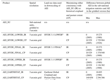
Table 1. Spatial resolution, land use data used in downscaling of area equipped for irrigation (AEI) compiled from sub-national statistics (AEI_SU), consistency rules in downscaling and AEI lost in downscaling for products in the global historical irrigation data set HID.
Product Spatial Land use data used Maximizing either Difference between global
resolution in downscaling of consistency with AEI in the sub-national
AEI AEI_SU (IR) or irrigation statistics and AEI
historical cropland in the gridded version (ha)
and pasture extent
(CP) Min Max
AEI_SU Sub-national n/a n/a n/a
units, gridded to 5 arcmin
AEI_HYDE_LOWER_IR 5 arcmin grid HYDE 3.1 LOWERa IR 0 19 275
(2005) (1980)
AEI_HYDE_LOWER_CP 5 arcmin grid CP 10 529 1 729 904
(2005) (1920)
AEI_HYDE_FINAL_IR 5 arcmin grid HYDE 3.1 FINALa IR 0 19 275
(2005) (1980)
AEI_HYDE_FINAL_CP 5 arcmin grid CP 10 529 1 378 940
(2005) (1900)
AEI_HYDE_UPPER_IR 5 arcmin grid HYDE 3.1 UPPERa IR 0 19 275
(2005) (1980)
AEI_HYDE_UPPER_CP 5 arcmin grid CP 10 529 1 136 382
(2005) (1900)
AEI_EARTHSTAT_IR 5 arcmin grid Earthstat Global IR 0 18 695
Cropland and (2005) (1980)
AEI_EARTHSTAT_CP 5 arcmin grid Pasture Data from CP 140 058 2 296 306
1700–2007b (2005) (1990)
aKlein Goldewijk et al. (2011),bhttp://www.earthstat.org.
to provide water to crops. It includes area equipped for full/partial control irrigation, equipped lowland areas, and areas equipped for spate irrigation (FAO, 2014a), but it ex-cludes rainwater harvesting. AEI is reported in many na-tional census databases and internana-tional databases such as FAOSTAT (FAO, 2014b), Aquastat (FAO, 2014a), or Eu-rostat (European Commission, 2014). For several countries with large extent of irrigated land (e.g. USA, India, Pakistan, Australia), statistics on AEI are not available because the corresponding national data centres only collect data on the area actually irrigated (AAI) during the year of the survey. In those cases AEI is often estimated based on AAI. AAI can be much lower than AEI when a part of the irrigation infrastruc-ture is not used, e.g. because the land is left fallow or because rainfed crops are cultivated. In the Natural Resource Inven-tory of the USA, for example, areas are considered irrigated when irrigation occurs during the year of inventory, or during ≥2 of the 4 years prior to the inventory (US Department of Agriculture, 2009). This resulted in an estimate of irrigated land for year 2007 that is 31 % larger than AAI reported by the agricultural census for the same year.
To ensure categorical consistency in reported variables, international databases such as Aquastat (FAO, 2014a) use similar methods to estimate AEI for countries where only AAI is available. In contrast, historical irrigation statistics or historical reports often simply refer to irrigated land with-out defining the term; therefore, comparisons with other data sources and knowledge of the statistics system in the corre-sponding country are required to infer whether AAI or AEI is meant. Although AAI differs from AEI, we also used statis-tics on AAI to develop this inventory because trends in AEI are often similar to trends in AAI. Furthermore, data on AAI at high spatial resolution were used to estimate the spatial pattern in AEI when AEI was only available at low resolu-tion. The methods used to estimate AEI based on AAI are described below (Sect. 2.1.3).
2.1.2 Description of input data and sources of information
administra-0% 25% 50% 75% 100%
1900
1910 1920 1930 1940 1950 1960 1970 1980 1985 1990 1995 2000 2005
Census
Irrigation data (sub-national level) Irrigation data (country level) Own estimates
GMIAv5
International organisation (eg FAO) 2nd hand data from literature Census
International organisation (eg FAO) 2nd hand data from literature Scaled sub-national value based on cropland extent
[image:4.612.129.463.66.288.2]Scaled based on neighbouring countries / own estimate / constant (in case of year 2005 no data available since year 2000) Interpolation / extrapolation
Figure 1. Overview of the types of input data used to develop the sub-national inventory of historical statistics on the area equipped for irrigation (AEI_SU) for the period 1900–2005. Please note that the spatial pattern of AEI_SU in 2005 is mainly determined by version 5 of the Global Map of Irrigation Areas GMIAv5 (Siebert et al., 2013), which again is based on sub-national irrigation statistics, mainly at the second or third administrative unit level.
tive unit boundaries. Major sources of historical statistics on AEI include the FAO databases Aquastat (FAO, 2014a) and FAOSTAT (FAO, 2014b). Both databases have reported AEI since 1961. While Aquastat only reports data for years with national surveys, FAOSTAT also contains expert esti-mates to fill the gaps between national surveys. FAOSTAT only contains data at the national level while Aquastat also reports data at the sub-national level. Another international database used in this study was Eurostat (European Com-mission, 2014) containing data on AEI (referred to as ir-rigable area in this database) for the European countries at sub-national level. Data for the years 1990, 1993, 1995, 1997, 2000, 2003, 2005, and 2007 were extracted from this database.
In addition to these international databases, we also used data collected in national surveys and derived from census reports or statistical yearbooks for most of the countries be-cause the spatial detail is often higher in national data sources than in the international databases. For the period before 1950, availability of national census data on AEI was limited to a few countries. Therefore, we also used secondary sources from the literature, e.g. scientific publications or books with reported data from primary national sources.
Many of the irrigation statistics for year 2005, as the start-ing point of the hindcaststart-ing, were derived from the database used to develop version 5 of the Global Map of Irrigation Areas (GMIA5). This data set, which is described in de-tail in Sect. 2.2.1, contains several layers describing AEI, AAI and the water source for irrigation at a global scale in 5 arcmin resolution (Siebert et al., 2013). We used the
data layer on AEI for downscaling the irrigation statistics to 5 arcmin grid cells (see Sect. 2.2); therefore, the sub-national irrigation statistics used to develop the GMIA5 data set were automatically incorporated into this HID. However, for many countries, the sub-national irrigation statistics used to develop the GMIA5 data set referred to a year different from 2005. Therefore, the difference between AEI in the year taken into account in GMIA5 and the year 2005 was derived from other sources, e.g. FAOSTAT, Eurostat or data derived from national statistical offices. For most of the years, be-tween 50 and 75 % of the global AEI was derived from sub-national statistics, most of it provided by reports of sub-national surveys (Fig. 1). The data sources are described in detail for each country and time step in Supplement S1.
or Germany, we used historical maps to create the adminis-trative area boundaries for the available data. For each time step we created a unique administrative boundary layer, de-pending on the level of data available for each country and changes in administrative units. These layers were converted to grids with 5 arcmin resolution and are provided as Supple-ment S2.
2.1.3 Methods used to harmonize data from different sources
For most of the countries, we used data derived from differ-ent sources with differdiffer-ent temporal and spatial resolution and sometimes different definitions used for irrigated land which resulted in inconsistencies among the input data sets (Supple-ment S1). Moreover, national irrigation surveys were often undertaken for years that differ from the time steps used in this inventory. This resulted in data gaps, which needed to be filled by interpolation or scaling. Therefore, it was important to harmonize the data, particularly within a country as well as among countries. The three main harmonising procedures were (i) data type harmonising, (ii) temporal harmonising, and (iii) infilling data gaps. These procedures are briefly in-troduced below with detailed information in Supplement S1 on procedures, assumptions, and data sources used for each country and time step.
– Data type harmonising was used when statistics referred to terms different from the definition used in this in-ventory for AEI. One example is China where the ir-rigated area reported in statistical yearbooks refers to the so-called effective irrigation area which includes an-nual crops but excludes irrigated orchard and pasture. In these situations we used the closest time step in which we had both data, AEI and the effective irrigation area or other terms used in original data sources, to calcu-late a conversion factor. This conversion factor was then applied at the sub-national level assuming that the ra-tio between AEI and the term reported in the original data source did not change over time. For other coun-tries, e.g. Argentina, Australia, India, Syria, the USA, or Yemen, the national databases referred to AAI. AEI was then estimated as the maximum of the AAI reported at high spatial resolution (e.g. county or district level) for different years around the reference year. Again a conversion factor (estimated AEI divided by reported AAI for the reference year) was calculated and applied to estimate AEI based on reported AAI for historical years. Data sources and procedures to estimate or derive AEI and AAI for each country around year 2005 are de-scribed in detail in the report documenting the develop-ment of GMIA5 (Siebert et al., 2013), while the method used for data type harmonising in historical years is de-scribed in Supplement S1.
– Temporal harmonising was used when the input data did not exactly correspond with the predefined time steps and thus data needed to be interpolated between years to match with the exact year in question. For this purpose we used a linear interpolation between the two closest data points on each side of the time step in question. – Filling of data gaps was required when irrigation
statis-tics were not available either for a specific time step or for the time step before or after. In this case we used, similar to the method applied for temporal har-monising, a linear interpolation between two existing data points, or we estimated AEI based on other infor-mation (e.g. trend in AEI in neighbouring countries, or trend in cropland extent). In cases where we had reli-able data from a neighbouring country, where irrigation development is known to be similar to the country in question, we used the trend in the neighbouring coun-try to scale the evolution of irrigation in that particular country. In some cases with gaps in sub-national data we used cropland extent development data to fill these gaps. We did this for example in China for years 1910–1930, where we used cropland development based on the His-tory Database of the Global Environment HYDE (Klein Goldewijk et al., 2011) to fill gaps in the sub-national data set (Buck, 1937) that did not have information for all of the provinces in China.
2.2 Downscaling of irrigation statistics to 5 arcmin resolution
The spatial database of sub-national irrigation statistics was developed as described in the previous section, including data on the AEI per country or sub-national unit and the corresponding geospatial data describing the administrative set-up (boundaries of national or sub-national units in each time step). To derive AEI on a 5 arcmin resolution and thus the final product of HID, additional data were required. Fur-ther, we developed a downscaling method to spatially allo-cate changes in AEI for each time step.
2.2.1 Data used for downscaling
As a starting point for the hindcasting in 2005 we used AEI data from GMIA5 (Siebert et al., 2013). This data set com-bines statistics on AEI for 36 090 sub-national administra-tive units with a large number of irrigation maps or remote-sensing-based land use inventories. The reference year dif-fered among countries, with about 90 % of global AEI as-signed according to statistical data from the period 2000– 2008. By using GMIA5 as a starting point for the downscal-ing, the underlying data were automatically introduced into the HID.
ex-tent of cropland and pasture. We demonstrate our method in this study by using cropland and pasture extent derived from version 3.1 of the History Database of the Global Environ-ment HYDE (http://themasites.pbl.nl/tridion/en/themasites/ hyde/index.html) and by using the Earthstat global crop-land and pasture data set developed by the Land Use and Global Environment Research Group at McGill University (http://www.earthstat.org/). Both data sets have a spatial res-olution of 5 arcmin and cover the period 10 000 BC–AD 2005 (HYDE) or 1700–2007 (Earthstat). The hindcasting method-ology developed in this study can be applied to any global historical data set if the extent of cropland and pasture is re-ported for the time steps considered in this study.
The HYDE cropland data set was developed by assigning cropland reported in historical sub-national cropland statis-tics to grid cells based on two weighting maps. One weight-ing map was based on satellite imagery and showed the crop-land extent in year 2000, while the second map was devel-oped by considering urban built-up areas, population den-sity, soil suitability for crops, extent of coastal areas and river plains, slope, and annual mean temperature. The in-fluence of the satellite map (first weighting map) increased gradually from 10 000 BC to AD 2005 while the impact of the second weighting map declined over time (Klein Gold-ewijk et al., 2011). Allocation of pasture to specific grid cells was similar but the second weighting map consid-ered additional information on the biome type (Klein Gold-ewijk et al., 2011). To account for uncertainties in histor-ical land use, mainly caused by assumptions on historhistor-ical per capita cropland and pasture demand, the HYDE database also provides upper and lower bounds on cropland and pas-ture use. Consequently, we used three HYDE versions as in-put data for our historical irrigation database: the best guess called HYDE_FINAL and the upper and lower estimates HYDE_UPPER and HYDE_LOWER resulting in separate gridded products of our historical irrigation database.
The Earthstat Global Cropland and Pasture Data 1700– 2007 represents a complete revision of the historical crop-land data set developed previously at the Center for Sus-tainability and the Global Environment (SAGE) at Univer-sity of Wisconsin-Madison (Ramankutty and Foley, 1999). Based on remote-sensing data and land use statistics, a crop-land and pasture map for year 2000 was created (Ramankutty et al., 2008). Historical (and future) changes in cropland and pasture extent were then estimated using a simple scaling ap-proach that combined the maps for year 2000 with historical (and future) sub-national cropland and pasture extent statis-tics and estimates, using the same method as Ramankutty and Foley (1999). The data have been made available by the Earthstat group (http://www.earthstat.org/). In the subse-quent sections we refer to the data set as EARTHSTAT.
2.2.2 Description of downscaling method
The objective of the downscaling procedure was to assign AEI to 5 arcmin grid cells and to ensure that the sum of the AEI assigned to specific grid cells is similar to the AEI re-ported by the sub-national statistics for the corresponding sub-national administrative unit and year. In addition, we wanted to ensure that for each grid cell AEI did not exceed the sum of cropland and pasture extent in that year. Further, irrigated land in the past is preferably assigned to grid cells where we find it presently. However, it was impossible to generate layers of historical irrigation extent that were com-pletely consistent with both the historical irrigation statistics and the historical cropland and pasture maps because of dif-ferences in methodology, input data, and assumptions used to generate the HID and the historical cropland and pasture maps. For some administrative units and years, for example, AEI is larger than the sum of cropland and pasture extent. Be-cause of spatial mismatch between AEI and agricultural land, these inconsistencies are even larger at the grid cell level. In many grid cells, AEI according to the GMIA5 exceeds the sum of cropland and pasture area in year 2005 according to the two historical land use inventories.
To account for these inconsistencies, we developed a step-wise approach to maximize the consistency with either the sub-national irrigation statistics (AEI_SU) or with the histor-ical cropland and pasture data (Fig. 2). Therefore, eight sep-arate time series of gridded data were developed which dif-fered with respect to the historical cropland and pasture data set used (HYDE_LOWER, HYDE_FINAL, HYDE_UPPER, or EARTHSTAT) and with regard to the consistency with ei-ther the sub-national irrigation statistics (suffix_IR) or with the historical land use (suffix CP) (Table 1, Fig. 2).
The downscaling procedure marched back in time start-ing with year 2005. A nine-step procedure was repeated for each sub-national statistical unit, each year in the time se-ries and each of the gridded products (Fig. 2). For each step and grid cell, a maximum irrigation area IRRImaxwas calcu-lated according to the criteria described in Fig. 2. The criteria were defined in a way that IRRImaxincreased with each of the nine steps by considering more and more areas outside the extent of irrigated land in the previous hindcasting time step. The basic assumptions underlying the rules shown in Fig. 2 are that irrigated areas in historical periods are more likely to occur at places where irrigated areas are today, that irrigation of cropland is more likely than irrigation of pasture and that irrigation of pasture is more likely than irrigation of non-agricultural land.
land area
irrigated land
cropland
cropland or pasture
S1 IRRImax = Min (IRRIt+1, CROP) IRRImax = Min (IRRIt+1, CROP)
S2 IRRImax = Min (IRRIt+1, CROP+PAST) IRRImax = Min (IRRIt+1, CROP+PAST)
S3 IRRImax = Min (IRRIt+1, LAND)
S4 IRRImax = IRRIt+1
S5 IRRImax = Max (IRRIt+1, CROP) IRRImax = Max (CROP, Area in S2)
S6 IRRImax = Max (IRRIt+1, CROP+PAST) IRRImax = CROP+PAST
S7 IRRImax = CROP if IRRIt+1=0
IRRImax = IRRImax from S6 if IRRIt+1>0
IRRImax = CROP if IRRIt+1=0
IRRImax = CROP+PAST if IRRIt+1>0
S8 IRRImax = Max (IRRIt+1, CROP+PAST) IRRImax = CROP+PAST
S9 IRRImax = Max (IRRIt+1, LAND)
In grid cells with
In all grid cells with:
in
time step t+1
Maximizing consistency with subnational irrigation statistics (AEI_SU)
Maximizing consistency with historical cropland and pasture
IRRI
[image:7.612.128.464.67.215.2]max
Figure 2. Illustration of the rules used to assign irrigated area to specific grid cells. The maximum irrigated area in each grid cell (IRRImax)
is calculated in steps S1–S9 depending on irrigated area assigned to the grid cell in the previous time step (IRRIt+1), cropland extent in the
current time step (CROP), pasture extent in the current time step (PAST) and total land in the grids cell (LAND). The assignment terminates, when the sum of IRRImaxfor all grids cells belonging to an administrative unit is greater than or equal to the irrigated area reported in the
sub-national statistics for the administrative unit. Please note that the previous time step ist+1 (and nott−1) as the procedure is marching back in time. The downscaling procedure is described based on seven examples in Supplement S4.
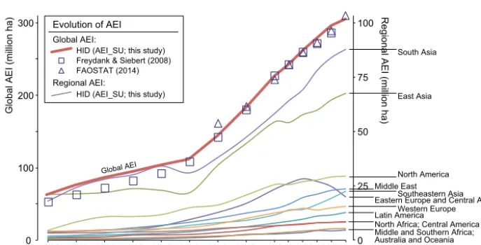
Global AEI
0 50
25 75 100
Global AEI (million ha)
0 100 200
300 Regional AEI (million ha)
1900 1910 1920 1930 1940 1950 1960 1970 1980 1985
1990 1995
2000 2005
Latin America
North Africa; Central America Middle and Southern Africa; Australia and Oceania
Western Europe Eastern Europe and Central Asia Southeastern Asia Middle East
North America East Asia South Asia HID (AEI_SU; this study)
HID (AEI_SU; this study) Freydank & Siebert (2008) FAOSTAT (2014) Global AEI:
Regional AEI:
Evolution of AEI
Figure 3. Evolution of regional (thin lines; rightyaxis) and global (thick line and symbols; leftyaxis) area equipped for irrigation (AEI) for the 20th century based on the sub-national historical irrigation statistics (AEI_SU) collected for the historical irrigation data set (HID), and of global AEI in Freydank and Siebert (2008) and FAOSTAT (FAO, 2014b).
in absolute terms (equal area in each grid cell). Performing half of the reduction as an area equal for each grid cell en-sured that cell-specific AEI became 0 in many grid cells with little AEI in the previous time step and that, consequently, the number of irrigated grid cells declined in the hindcasting process. Different from the national scaling approach, the de-crease of irrigated area in each grid cell is not the same within a sub-national unit because in step 1 of the downscaling ap-proach, information on cropland area in the grid cell at timet
is also taken into account (Fig. 2).
When the sum of IRRImax in the administrative unit cal-culated for a specific step was less than the AEI reported in the historical database, AEI in each grid cell was set to IRRImaxand the routine proceeded to the next step. The
pro-cedure was terminated and the subsequent steps discontin-ued when the sum of IRRImaxin the administrative unit ex-ceeded the AEI_SU reported in the historical database. Half of the increment in AEI still required in the present step was assigned in relative terms (equal fraction of the grid-cell-specific IRRImax after the previous step) and the other half of the required increment was assigned as an area equal for each grid cell. The downscaling procedure is explained in more detail in Supplement S4 where we describe the specific steps and calculations using seven examples.
[image:7.612.128.472.308.483.2]with AEI_SU (Fig. 2). The gridded products maximiz-ing consistency with historical cropland and pasture ex-tent (AEI_HYDE_LOWER_CP, AEI_HYDE_FINAL_CP, AEI_HYDE_UPPER_CP, AEI_EARTHSTAT_CP) ensured that AEI was less than or equal to the sum of cropland and pasture extent, for each time step and grid cell. There-fore, the AEI in the gridded products is less than the AEI reported in the sub-national statistics for administra-tive units in which AEI_SU exceeded the sum of crop-land and pasture extent (Table 1). In the gridded products maximizing consistency with the historical irrigation statis-tics (AEI_HYDE_LOWER_IR, AEI_HYDE_FINAL_IR, AEI_HYDE_UPPER_IR, AEI_EARTHSTAT_IR) AEI can exceed the sum of cropland and pasture extent. Therefore, the AEI reported in the sub-national irrigation statistics was completely assigned to the gridded products (Table 1), with the exception of a few administrative units that were so small that they disappeared in the conversion of the administra-tive unit vector map to 5 arcmin resolution grids (mainly very small islands).
2.3 Methods used to analyze the data set
2.3.1 Comparison of the historical irrigation database with other data sets and maps
Validation of HID against historical statistical data was not possible because all historical irrigation statistics available to us were used as input data to develop the HID. However, we compared our spatial database of sub-national irrigation statistics to AEI reported in other inventories at the national scale to highlight the differences (FAO, 2014b; Freydank and Siebert, 2008).
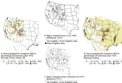
We found two historical maps showing the major irriga-tion area in the western part of the USA in year 1909 (Whit-beck, 1919) and year 1911 (Bowman, 1911) and compared our 5 arcmin irrigation map for year 1910 visually with these two maps. In addition, we compared our map to a global map showing the extent of the major irrigation areas and in-terspersed irrigated land beginning of the 1960s (Highsmith, 1965). A strict numerical comparison was not useful because the way irrigated land is shown on these maps is incom-patible with our product. Historical irrigation maps include shapes of regions in which major irrigation development took place, resulting in a binary yes or no representation (see also the maps shown in Achtnich, 1980; Framji et al., 1981–1983; Whitbeck, 1919). But even within the areas shown on these maps as irrigated there were sub-regions that were not irri-gated (e.g. buildings, roads, rainfed cropland or pasture). In addition, many minor irrigation areas with small extent were not represented on these maps because of the limited accu-racy of the historical drawings (Highsmith, 1965). In con-trast, the gridded product developed in this study shows the percentage of the grid cell area that is equipped for irriga-tion and thus provides a discrete data type. Therefore a visual
comparison was preferred to a numerical one. We also com-pared our new product (HID) to maps derived by multiply-ing the GMIA5 with scalmultiply-ing factors derived from historical changes in AEI at country level, as this procedure has been used in previous studies (Puma and Cook, 2010; Wisser et al., 2010; Yoshikawa et al., 2014).
2.3.2 Gridded area equipped for irrigation in the different product lines
Differences in AEI across gridded products were evaluated by pair-wise calculation of cumulative absolute differences (AD) (ha) as
AD=
n
X
c=1
|AEI_Ac−AEI_Bc|, (1)
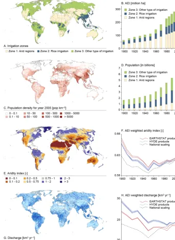
Figure 4. (a) Classification of irrigation areas in dry areas, wet rice cultivation areas, and other wet irrigation areas and (b) development of global AEI for historical irrigation data set (HID; AEI_HYDE_FINAL_IR) in these zones for the period 1900–2005; (c) population density for year 2005 according to the HYDE database (Klein Goldewijk et al., 2010) and (d) number of people in the three different irrigation zones in the period 1900–2005; (e) aridity index according to the CGIAR-CSI Global Aridity and ET database (CGIAR-CSI, 2014; Zorner et al., 2008) and (f) change in mean aridity on irrigated land in the period 1900–2005; (g) mean annual river discharge in the period 1961–1990 calculated with WaterGAP 2.2 (Müller Schmied et al., 2014) and (h) change in global mean of natural river discharge on irrigated land in the period 1900–2005.
cells with an aridity index greater than 0.65 and a harvested area of irrigated rice that was at least 30 % of the total har-vested area of irrigated crops according to the MIRCA2000 data set (Portmann et al., 2010). To fill the gaps between grid cells that are not irrigated according to MIRCA2000
[image:9.612.126.469.71.542.2]irrigation is mainly used to increase crop yields by reduc-ing drought stress durreduc-ing occasional dry periods. We calcu-lated the change in AEI in the three zones at the global scale and in addition the number of people in the distinct irriga-tion zones based on the HYDE populairriga-tion density (Fig. 4c) (Klein Goldewijk, 2005).
2.3.4 Change in climatic water requirements and freshwater availability in areas equipped for irrigation
As a final step in analysing our gridded historical irriga-tion maps, we calculated the change in mean aridity and mean natural river discharge on irrigated land as indicators of changes in climatic water requirements and freshwater avail-ability for irrigation. Global means were derived for both indicators. Mean aridity on irrigated land was computed by weighting cell-specific aridity with AEI within the cell as
AI=
n5
X
c=1
AIc·AEIc !
/AEI, (2)
where AI is the mean aridity index on irrigated land (–), AIc is the aridity index in grid cellcderived from the CGIAR-CSI Global Aridity and PET Database (Fig. 4e) (CGIAR-CSI, 2014; Zorner et al., 2008), AEIcis the AEI in cellc(ha), AEI is the total AEI (ha), andn5 is the number of 5 arcmin grid cells with irrigation.
Similarly, mean natural river discharge on irrigated landQ
(km3yr−1) was calculated as
Q=
n30
X
c=1
Qc·AEIc !
/AEI, (3)
whereQc is the mean annual river discharge in the period 1961–1990 (Fig. 4g) (km3yr−1) calculated with the global water model WaterGAP 2.2 (Müller Schmied et al., 2014) at a 30 arcmin resolution by neglecting anthropogenic water ex-tractions and by using GPCC precipitation and CRU TS3.2 (Harris et al., 2014) for the other climate input data, andn30 is the number of 30 arcmin grid cells with irrigation. To per-form these calculations on a 30 arcmin grid, the historical ir-rigation maps were aggregated as described in Sect. 2.3.2.Q
in this study refers to the entire river discharge that would be potentially available for the irrigated areas if there were no human water abstractions in the upstream basin.
3 Results
3.1 Irrigation evolution over the 20th century
The pace of irrigation evolution can clearly be divided into 2 eras, with the year 1950 being the breakpoint. Prior to 1950, the AEI gradually increased, whereas since the 1950s the AEI increased extremely rapidly until the end of the century
before somewhat levelling off within the first 5 years of the 21st century (Fig. 3). According to the AEI_SU of the HID database, the global AEI covered an area of 63 Mha in year 1900, nearly doubled to 111 Mha within the first 50 years of the 20th century and approximately tripled within the next 50 years to 306 Mha by year 2005 (Fig. 3).
More variation can be seen in the historical trends when those are explored for regions or countries separately (Fig. 3, Table A1). In many regions irrigation increased more rapidly (relative to year 1950) than the global average since the 1950s (most rapidly in Australia and Oceania, southeast-ern Asia, Middle and South Africa, Central America, and eastern Asia), while irrigation development has been much slower than the global average in North America and North Africa. AEI development in eastern Europe and central Asia is unique, with a slow decrease due to the collapse of the former irrigation infrastructure since 1990.
When AEI is compared across world regions, South Asia and eastern Asia have had the largest shares in global irriga-tion over the entire study period, ranging from 26 to 33 and 20 to 34 %, respectively (Supplement S3). Other world re-gions with substantial AEI include North America, Mid-dle East, eastern and central Asia, and Southeast Asia, with shares on global AEI between 7 and 12 %.
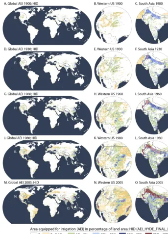
AEI at the grid cell level in year 1900 shows concentra-tions of irrigated land mainly on arid cropland, e.g. west-ern North America, the Middle East and central Asia, along the Nile and Indus rivers or the upstream region of the river Ganges (Figs. 4e and 5a). In China, Japan, Indone-sia and western Europe irrigated land was mainly in humid regions and served watering of rice fields (Asia) or mead-ows (western Europe). In Africa, important irrigation in-frastructure was found only in Egypt and South Africa. In eastern Europe, the extent of irrigated land was limited to the southern part of Russia and the Ukraine (Fig. 5a). In 12 countries the extent of irrigated land exceeded 1 Mha in the year 1900: India (17.8 Mha), China (17.6 Mha), the USA (4.5 Mha), Japan (2.7 Mha), Egypt (2.3 Mha), Indone-sia (1.4 Mha), Italy (1.3 Mha), Kazakhstan (1.2 Mha), Iran (1.2 Mha), Spain (1.2 Mha), Uzbekistan (1.1 Mha), and Mex-ico (1.0 Mha) (Supplement S3).
Figure 5. Spatial and temporal evolution of global area equipped for irrigation (AEI) for five time steps (1900, 1930, 1960, 1980, and 2005) based on the product AEI_HYDE_FINAL_IR of the historical irrigation data set (HID). The maps are presented at global scale and for two selected close-up areas, namely western USA and South Asia, for each time step.
Bangladesh, southern India, Malaysia, Myanmar, North and South Korea, the Philippines, Sri Lanka, Thailand, and Viet-nam (Supplement S3, Fig. 5g).
Until year 1980 AEI continued to increase, reaching its maximum extent in some countries in eastern Europe, Africa, and Latin America (Belarus, Bolivia, Botswana, Estonia, Hungary, Mozambique, and Poland) (Fig. 5j). Until year 2005 AEI increased further in many countries and extended also to the more humid eastern part of the USA (Fig. 5).
Mauritania, Mozambique, South Korea, and Taiwan (Supple-ment S3).
3.2 Gridded area equipped for irrigation in the different gridded products
The rules used to downscale AEI_SU to grid cells (Fig. 2) resulted in differences in AEI per grid cell but also in dif-ferences in the total AEI assigned in total in the gridded products. The main reason is that AEI in each grid cell was constrained to the sum of cropland and pasture for the prod-uct lines that maximize consistency with the land use data sets (right column in Fig. 2, see Sect. 2.2.2). In particular in very small sub-national administrative units in arid regions, where most of the agricultural land is irrigated, AEI based on irrigation statistics was larger than the sum of cropland and pasture in the corresponding administrative unit. Conse-quently, in the downscaling process this difference between AEI and the sum of cropland and pasture was not assigned to grid cells. In the product lines maximizing consistency with the irrigation statistics (left column in Fig. 2) AEI was constrained by total land area only. Therefore, if required (in step 9 of the allocation), AEI exceeded the sum of cropland and pasture. In the gridded products based on HYDE land use the AEI not assigned to grid cells was smallest in year 2005 (10 529 ha or 0.003 % of total AEI) and largest in year 1900 (2.6 % of total AEI in AEI_HYDE_LOWER_CP, 2.1 % of total AEI in AEI_HYDE_FINAL_CP, and 1.6 % of total AEI in AEI_HYDE_UPPER_CP). In AEI_EARTHSTAT_CP, the extent of AEI not assigned to grid cells was largest in year 1990 (2.3 Mha) while the extent relative to total AEI was largest in year 1920 (0.9 %).
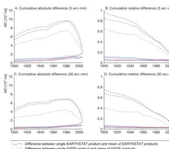
While differences in total AEI per administrative unit across gridded time series are relatively low, differences at the grid cell level are considerable (Supplement S5). This reflects different patterns in historical cropland and pasture extent and varying downscaling rules. Cumulative absolute differences, calculated according to Eq. (1), increase in the hindcasting process from 2005 to 1970 and decrease prior to that until year 1900 (Fig, B2a and c). In contrast, relative dif-ferences are lowest in year 2005 and increase continuously until year 1900 (Fig. B2b and d). Differences among the six gridded products based on HYDE land use are relatively low, similar to differences among the two products based on EARTHSTAT land use. In contrast, differences between the specific gridded products and the mean of all gridded prod-ucts are much larger but still lower than the difference be-tween the mean of the gridded products of the HID and AEI derived from the national scaling approach (Fig. B2).
Thus, differences between the HYDE land use and the EARTHSTAT land use seem to have a larger effect than dif-ferences between the HIGHER, LOWER and FINAL HYDE land use variants. Aggregation of the data to 30 arcmin reso-lution reduced AD and RD by about one-third (Fig. B2) but differences at the grid cell level are considerable even at this
resolution. This shows the importance of using different land use data sets for the development of historical irrigation data and the need to develop specific gridded products to be used in conjunction with specific cropland and pasture data sets. To describe and map our results in more detail, for the next sections we used the product AEI_HYDE_FINAL_IR which has maximum consistency with the sub-national irrigation statistics.
3.3 Irrigation evolution by irrigation category
In year 1900 about 48 % of the global AEI was in dry ar-eas, 33 % in wet areas with predominantly rice irrigation and 19 % in other wet areas (Fig. 4b). In contrast, only 19 % of the global population lived in dry regions while 35 % of the global population lived in wet areas with predominantly rice irrigation and 46 % in other wet areas (Fig. 4d). The reason for differences between AEI and population in these zones is likely that the majority of the rainfed cropland was located in wet regions whose carrying capacity without irrigation was higher and consequently a higher population density could be supported. While the share of AEI in dry regions remained quite stable varying around 50 % through the entire study period (e.g. 46 % in year 2005 and 48 % in year 1900), the share of AEI in wet regions with predominantly rice irriga-tion decreased from 33 to 26 % while the share of AEI in other wet irrigation areas increased from 19 to 28 % between 1900 and 2005 (Fig. 4b). The share of the global population living in dry regions increased between 1900 and 2005 from 19 to 26 % while the population living in other wet regions decreased from 46 to 35 % (Fig. 4d).
3.4 Change in mean aridity and river discharge in areas equipped for irrigation
The global mean aridity index on AEI declined from year 1900 to 1950 from 0.66 to 0.60 indicating that new irriga-tion was developed on land with higher aridity. After 1950 the mean aridity index increased to 0.63 until year 2005 (Fig. 4f). Global mean natural river discharge on AEI de-clined by 4–5 km3yr−1 in the period 1900–1950 (EARTH-STAT and HYDE gridded products) and increased then again by 2 km3yr−1(7.8 %) (EARTHSTAT products) or remained more or less stable (HYDE products) (Fig. 4h). For 2005, all products converge to a mean natural river discharge on irri-gated land of 24–25 km3yr−1.
4 Discussion
4.1 Data set comparison
between 1900 and 2000. However, for several countries the AEI_SU data used for the HID differ from those in the two other inventories (Tables A1 and A2).
There are three major reasons for these differences be-tween HID and FAOSTAT:
First, there are countries in which statistics on AEI are not collected by the official statistics departments such as Aus-tralia, Canada, New Zealand, Pakistan, and Puerto Rico. In these countries statistics on irrigated land refer to the AAI in the year of the survey. Many factors can result in only a part of the irrigation infrastructure being actually used for irrigation, such as failure in water supply or damaged infras-tructure. In other, mainly humid and sub-humid regions, only specific high value crops, such as vegetables, are irrigated (Siebert et al., 2010). For many of these countries FAOSTAT reports the AAI instead of AEI while the statistics used for the HID were adjusted (as described in Sect. 2.1.3) to account for the difference between AEI and AAI. Consequently, AEI in the HID is higher than the irrigated area reported by FAO-STAT (Table A1).
Another group of countries in which AEI in the HID differs from the data reported by FAOSTAT is devel-oped regions, e.g. in Europe, North America or Ocea-nia, such as Austria, Canada, Germany, Greece, Italy, Portugal. FAO is collecting detailed country-specific in-formation on water management and irrigation in its Aquastat program and provides this information in coun-try profiles (http://www.fao.org/nr/water/aquastat/countries_ regions/index.stm). These country profiles are based on in-formation obtained from different national data sources and are compiled and revised by FAO consultants from the re-spective country. This detailed information collected in the Aquastat program is also used to improve and update the time series in FAOSTAT. The mandate of FAO is, however, focused on developing and transition countries; therefore, these detailed country profiles are not available for devel-oped countries and consequently, less effort is made to im-prove historical data for these countries. In contrast, for many of the developed countries, the HID is based on information obtained from historical national census reports (Table A1).
A third group of countries with differences between AEI in the HID and FAOSTAT are the former socialist coun-tries in eastern Europe. In these councoun-tries large-scale irriga-tion infrastructure was developed with centralized manage-ment structure. After the transition to a market-based econ-omy, most of this former infrastructure was not used any-more and it is a matter of definition to decide whether these areas should still be considered as areas equipped for irri-gation or not. For most of these countries the HID shows a major decline in AEI after 1990 (based on national surveys or statistics on irrigable area provided by Eurostat) while FAOSTAT still includes the former irrigation infrastructure in some countries (Table A1).
The main reason for differences between AEI per country in the HID and the inventory of AEI per country (Freydank
and Siebert, 2008) (Table A2) is that the number of refer-ences used to develop the HID was much larger than the num-ber of historical reports used by Freydank and Sienum-bert (2008). Many assumptions used in Freydank and Siebert (2008) were thus replaced by real data. This also includes changes for the year 2000 (e.g. for Australia, Bulgaria, Canada, China, Indonesia, Kazakhstan, Russia, Ukraine, and the USA; see Table A2) because the recent extent of irrigated land in Frey-dank and Siebert (2008) was based on the statistical database used to develop version 4 of the Global Map of Irrigation Ar-eas (Siebert et al., 2007), while the HID is consistent with the updated and improved version 5 of this data set (Siebert et al., 2013). In addition, the HID explicitly accounts for the histor-ical practice of meadow irrigation used mainly in central and northern Europe resulting in higher estimates of AEI, in par-ticular for year 1900 for many European countries, e.g. Aus-tria, Germany, Norway, Poland, Sweden, Switzerland, and UK (Table A2).
To verify the spatial patterns in historical irrigation ex-tent in the gridded product, we compared the product AEI_HYDE_FINAL_IR for year 1910 (Fig. 6a) to two his-torical maps of the major irrigation areas in the United States in years 1909 (Fig. 6b) and 1911 (Fig. 6c). We found that our product represents remarkably well the spatial pattern of the major irrigation areas shown on the historical maps, in par-ticular in states such as Idaho, Utah, and Wyoming. In some states, the pattern of AEI in the HID differs from the pattern shown in the historical maps. This can be expected because of the simplicity of our downscaling approach and because of difficulties of showing minor irrigation sites on the histor-ical maps. However, based on visual comparison of the maps it seems that for many states the agreement is even better than the match between the two historical maps, and that the agreement of the pattern shown in the HID and in the map for year 1909 is best. One exception is California where the HID and the historical map for year 1911 show irrigation devel-opment over the entire Central Valley (Fig. 6a and c) while in the historical map for year 1909 only shows irrigation in the southern part of the Central Valley (Fig. 6b).
agree-Figure 6. Comparison of the historical irrigation data set (HID) for year 1910 (developed using HYDE land cover, central estimate; AEI_HYDE_FINAL_IR) (a) with a map showing irrigated area in the western part of the USA in year 1909 (Whitbeck, 1919) (b), a map showing irrigated area in the western part of the USA in year 1911 (Bowman, 1911) (c), and an irrigation map for year 1910 developed by multiplying area equipped for irrigation (AEI) in year 2005 with scaling factors derived from historical changes of AEI at country level (d).
ment of the historical irrigation map (Highsmith, 1965) and our gridded product for year 1960 (AEI_HYDE_FINAL_IR) was found for the major irrigation areas in the Central Val-ley in California, along the Yakima River in Washington, at the High Plains aquifer in Texas, along the Colorado River and the Rio Grande (the United States, Mexico) in Alberta (Canada), the Pacific Coast and along Rio Lerma in Mexico, in Honduras and Nicaragua, in Peru, Chile and Argentina, in Spain, along the French Mediterranean coast, in northern Italy, Bulgaria and Romania, along the Nile River in Egypt and Sudan, in South Africa and Zimbabwe, in the Euphrates– Tigris region and the Aral Sea basin, in Azerbaijan, Pakistan, northern India and eastern India, in the area around Bangkok (Thailand), in Vietnam, Taiwan, North Korea, South Korea and Japan, in the North China Plain, on the island of Java (Indonesia), in the Murray–Darling Basin (Australia), and on the southern island of New Zealand (Supplement S6). However, there are also some regions that show differences in the two products. For example, the map published by Highsmith (1965) shows very little irrigation in the eastern United States, northern and central Europe, Portugal, south-west and northern France, southern Brazil, the Fergana Val-ley in Uzbekistan, the interior of Turkey, western China and Sumatra (Indonesia), while the sub-national statistics used to develop the HID indicate that there was irrigation already developed at this time (Supplement S6). For other regions,
such as northeast Brazil or Namibia, the extent of irrigated land seems to be larger in the historical drawings relative to the newly developed HID (Supplement S6). The general im-pression from the comparison of the two map products is that there is a very good agreement for most of the major irriga-tion areas while there is less agreement for the minor irri-gation areas. Some of the differences may be related to dif-ficulties with drawing interspersed small-scale irrigation on the historical maps. In other cases it may be that the newly developed HID shows irrigation in areas where infrastructure was not developed at this time, e.g. because the resolution of the sub-national irrigation statistics was not sufficient. 4.2 Improvements in mapping of historical irrigation
extent by the new inventory
[image:14.612.101.500.66.335.2]Figure 7. Comparison of the historical irrigation data set (HID) (developed using HYDE land cover, central estimate; AEI_HYDE_FINAL_IR) (a, c, e) to irrigation maps developed by multiplying area equipped for irrigation (AEI) in year 2005 with scaling factors derived from historical changes of AEI at country level (b, d, f) for years 1900 (a, b), 1960 (c, d) and 1980 (e, f).
improves on the historical development of irrigated land from previous studies by considering sub-national data on the ex-tent of irrigated land. In addition, when irrigated land de-clined historically, the number of irrigated grid cells is re-duced and irrigated land is concentrated into smaller regions in the HID (Figs. 6a, 7a, c and e) while there were many ir-rigated cells with very small irir-rigated areas in the historical layers when the national scaling approach was used (Figs. 6d and 7b–d).
At least for the USA, the historical pattern derived with the new method (HID) agrees much better with the pattern shown on historical maps (Fig. 6), particular in central US states (e.g. Texas, Kansas, and Nebraska). In the USA, irri-gation developed first in the arid western part of the country. While this is reflected well in the HID, a national scaling approach would also assign irrigated land to grid cells that are currently irrigated and located in the eastern part of the country, e.g. to the lower Mississippi Valley (Figs. 6 and 7). Similar to this, historical irrigated land in India was mainly located in the northwest of the country and in China more in the south of the country, while the national scaling approach would also assign irrigated land to the eastern part of India and the northeast of China (Fig. 7). Consideration of sub-national statistics therefore resulted in a clear improvement
in the historical irrigation layers, in particular for these large countries.
irriga-Figure 8. Ratio between the area equipped with irrigation according to the sub-national irrigation statistics (AEI_SU) used for the historical irrigation data set (HID) and cropland extent (a–c) or total cropland productivity (kcal ha yr−1, d–f) per country for years 1970 (a, d), 1990 (b, e) and 2005 (c, f); fraction of AEI in regions with mainly rice irrigation (g), mean aridity weighted with AEI (h), and mean river discharge weighted with AEI (km3yr−1, I). Cropland productivity (kcal ha−1yr−1) was calculated based on crop production data for years 1969–1971 (d), 1989–1991 (e) and 2004–2006 (f) and cropland extent for years 1970, 1990 and 2005 extracted from the FAO FAOSTAT database (FAO, 2014b).
tion water use, water scarcity, terrestrial water flows, or crop productivity.
4.3 Determinants of the fraction of irrigated cropland The indicators including AEI by irrigation category, change of mean aridity and of mean river discharge in AEI presented in Sect. 3.3 and 3.4 can also be associated with the fraction of irrigated cropland to better describe reasons for spatial dif-ferences in densities of irrigated land and of trends in irri-gation development (Fig. 8). Irriirri-gation is a measure of land use intensification because it is used to increase crop yields (Siebert and Döll, 2010). Therefore, a high density of irri-gated land can be expected in regions where high crop yields (in kcal per ha and year) are required to meet the demand for food crops due to high population densities, e.g. in South Asia, East Asia, and Southeast Asia (compare Fig. 8c and f). Consequently, a large part of the spatial patterns in the use of irrigated land can be explained by population density (Neu-mann et al., 2011). However, there are also other methods of land use intensification, e.g. multiple cropping, fertilization,
or crop protection from pests. The highest benefit from us-ing irrigation is achieved in arid and semi-arid climates be-cause of the reduction of crop drought stress and in paddy rice cultivation because rice is an aquatic crop and irrigation is also used to suppress weed growth by controlling the wa-ter table in the rice paddies. The high aridity explains the high fraction of irrigated cropland in central Asia, on the Arabian Peninsula, in Egypt, Mexico, the USA, Peru, and Chile (compare Fig. 8c and h) while the importance of tradi-tional paddy rice explains high fractions of irrigated cropland in tropical regions, e.g. in Southeast Asia, Suriname, French Guyana, Colombia, or in Madagascar and Japan (compare Fig. 8c and g).
[image:16.612.50.548.64.375.2](Fig. 8i). In contrast, annual discharge weighted with AEI is high in most of the humid rice cultivation regions (compare Fig. 8g and i) and in some regions where arid irrigation areas (Fig. 8h) are connected by a river to more humid upstream ar-eas (Fig. 8i), e.g. the river Nile basin in Egypt, the Indus and Ganges basins in Pakistan and India, the Aral basin in cen-tral Asia, or the Tigris and Euphrates basins in Turkey and Iraq. Many of the historical cultivation in these regions ben-efited greatly from irrigation and abundant water resources (Fig. 8a). In contrast, trends in the share of irrigated cropland between 1970 and 2005 (Fig. 8a–c) seem to be more closely associated with changes in cropland productivity, shown here as kcal produced per year and hectare of cropland (Fig. 8d– f). Large increases in cropland productivity in South Amer-ica, Southeast Asia, Mexico, the USA, and parts of western Europe (Fig. 8d–f) are consistent with increases in irrigated cropland fraction (Fig. 8a–c) while regions with a decline in irrigated cropland fraction, e.g. in the period 1990 to 2005 in eastern Europe, some countries of the former Soviet Union or Mongolia (Fig. 8b and c) agree with regions with a similar trend in crop productivity (Fig. 8e and f).
The relationships between irrigated cropland fraction and cropland productivity, aridity, rice cultivation, and river dis-charge raise the question of whether these relationships can be used to predict future spatio-temporal changes in the ex-tent of irrigated land. Such information could improve cli-mate impact assessments or global change studies, which as-sume in most cases a fixed extent of irrigated land in the com-ing decades. A key question for such applications will be to determine the drivers of land productivity. In historical peri-ods the majority of crops were produced close to the region of consumption; therefore, cropland productivity was mainly driven by population density (Boserup, 1965; Kaplan et al., 2011). More recently, regions of crop production and con-sumption are increasingly decoupled by trade flows (Fader et al., 2013; Kastner et al., 2014). World food supply has in-creased within the last 50 years but food self-sufficiency has not improved for most countries (Porkka et al., 2013). Fur-thermore, only a few countries, such as the USA, Canada, Brazil, Argentina, or Australia have been net food exporters while most other countries have been net food importers (Porkka et al., 2013). Most of these net food exporting coun-tries are characterized by an increase in cropland productiv-ity and irrigated land (compare Fig. 8d–e to Fig. 3 in Porkka et al., 2013). These net food exporting countries also supply crop products to net importing countries with low cropland productivity and a low extent of irrigated land, e.g. in Africa. In a globalizing world these long distance links are expected to become even stronger and need to be considered when pro-jecting future extent of irrigated land.
4.4 Limitations and recommended use of the data set The uncertainty in estimated AEI is driven by uncertainties in input data (statistics on AEI, cropland and pasture
ex-tent) and by the assumptions made when harmonizing input data or when disaggregating AEI per administrative unit to grid cells. In particular, for the period before 1960 availabil-ity of survey-based first-hand statistics on AEI was limited and missing data had to be replaced by expert guesses or assumptions (Fig. 1). Therefore, AEI for the period before 1960 is expected to be less accurate than afterwards. Similar to this, the trend for the development of global AEI maybe less certain for the most recent years in the time series be-cause detailed agricultural census surveys are typically un-dertaken only every 5–10 years and there is an additional 2– 5-year lag before the survey results become available. For many countries the latest detailed survey data were available for the period around year 2000 and sometimes it was as-sumed that AEI did not change afterwards until year 2005 (Supplement S1). Therefore the declining increase of AEI for the period 1998–2005 (Fig. 3) could be an artefact of the data constraints for the most recent years. Data availability also differed across countries (Supplement S1). In addition, boundaries of nations have been changing, for example, AEI for countries belonging to the former Soviet Union or the former Socialist Federal Republic (SFR) of Yugoslavia is re-ported since the begin of the 1990s, while for the period be-fore 1990 the trend in AEI was estimated based on the trend reported for the USSR or for the SFR of Yugoslavia unless sub-national information for historical years could be used. These changes in the extent of nations add another source of uncertainty to AEI.
Uncertainty in input data also impacts disaggregation of AEI into 5 arcmin resolution. In countries with a high reso-lution of sub-national irrigation statistics, uncertainty in the gridded product lines is expected to be less than in coun-tries where data are available at the national scale only, in particular in the case of large countries. The resolution of sub-national irrigation statistics has also been higher for the more recent time steps (Supplement S2). In the disaggre-gation process, sub-national irridisaggre-gation statistics were com-bined with gridded land use data sets (Sect. 2.2). There-fore, uncertainties in these input data are also introduced into the gridded product lines described in this article. Further-more, it is possible that the census-based land use statistics used as input to develop the HYDE and EARTHSTAT data layers on cropland and pasture extent may be inconsistent with the irrigation statistics used in this study, in particular for small sub-national statistical units. This issue cannot be avoided because often the institutions responsible for collect-ing land use data (e.g. Ministries of Agriculture) differ from institutions collecting irrigation data (e.g. Ministry of Water Resources; Ministry for Environment) resulting in different sampling strategies and different survey years.
fodder; therefore, the rule to preferentially assign irrigation to cropland (S1, S5, S7 in Fig. 2) resulted in incorrect assign-ment of irrigation in some places. The disaggregation could therefore be improved by applying country-specific disaggre-gation rules; these rules should also be time specific to reflect time-varying differences in irrigation infrastructure develop-ment across regions. However, the country-specific informa-tion on the historical development of irrigainforma-tion was insuffi-cient to develop these rules for this global-scale study.
Differences in spatial pattern of disaggregated AEI among the gridded products based on HYDE cropland and pasture extent and EARTHSTAT cropland and pasture extent suggest that the products developed in this study are only compatible with the specific land use data set used in this study as input. Application in studies in which both land use and irrigation data are required as input may result in inconsistencies when other land use information is used. However, the method and rules applied here are sufficiently general that they can easily be applied on request for other land use data sets reporting the extent of cropland and pasture at the required spatial and temporal resolution.
Because of differences in AEI at the grid cell level among the gridded products, we suggest that more than one specific gridded product should be used in typical applications such as global hydrological modelling to get a better understand-ing of differences in model outputs caused by usunderstand-ing different input data. We cannot make a general recommendation on which HID product may be most appropriate for different applications or represents patterns in AEI in a region better at this stage. When complete coverage of the global irrigation extent is most important, use of AEI_HYDE_FINAL_IR or AEI_EARTHSTAT_IR is recommended. When, in contrast, consistency with cropland or pasture data is more important, the corresponding CP-product (AEI_HYDE_LOWER_CP,
AEI_HYDE_FINAL_CP, AEI_HYDE_UPPER_CP,
AEI_EARTHSTAT_CP) may be more appropriate.
We are unable to quantify the uncertainties in our map be-cause this would require defining error ranges and probabili-ties for each specific source of uncertainty, e.g. all the sources used as input. However, we expect that uncertainties are scale dependent with higher uncertainty for specific grid cells than for entire countries or the whole globe and that estimates for specific years are less certain than trends for longer time pe-riods. Therefore, we recommend application of the data set mainly for global-scale research or for continental studies. Use of the data set for studies constrained to single countries is only suggested after carefully checking the resolution and origin of the input data used for the specific country (Sup-plement S1), checking the assumptions made to fill data gaps (Supplement S1), and testing whether the rules and assump-tions made in the downscaling (Fig. 2) are appropriate for that specific case.
The data set presented in this study shows AEI and we need to highlight that the spatio-temporal patterns in the de-velopment of AEI cannot directly be translated into patterns
5 Conclusions
Appendix A: Tables
Table A1. Area equipped for irrigation (AEI) compiled from sub-national statistics (AEI_SU) in the historical irrigation data set (HID) and the FAOSTAT database (FAO, 2014b) for years 1960, 1980, and 2005 (ha). Only countries with considerable differences between AEI in HID and FAOSTAT are shown. Units are ha. Data provided by FAOSTAT (FAO, 2014b) refer to country names and country boundaries in the year of reporting while the subnational statistics of the HID refer to the current administrative setup. Data shown in italic refer to aggregated administrative units contained in FAOSTAT, e.g. the Territory of former Czechoslovakia. To allow a comparison between HID and FAOSTAT, the sum of AEI for the disaggregated units, e.g. Czech Republic and Slovakia, was computed for the data contained in the HID.
Country HID HID HID FAOSTAT FAOSTAT FAOSTAT
1960 1980 2005 1961 1980 2005
Australia 1 345 292 2 358 248 3 993 255 1 001 000 1 500 000 2 545 000
Austria 41 429 60 000 119 430 4 000 10 000 120 000
Canada 343 850 858 581 1 200 586 350 000 596 000 845 000
Ghana 13 750 20 000 59 000 6 000 6 000 33 000
Greece 563 702 961 000 1 593 780 430 000 961 000 1 593 780
Hungary 77 063 431 333 152 740 133 000 134 000 152 750
Italy 2 428 139 3 500 000 3 972 660 3 400 000 3 400 000 3 973 000
Mozambique 51 667 120 000 118 120 8 000 65 000 118 000
New Zealand 215 607 441 739 607 462 77 000 183 000 533 000
Pakistan 10 649 990 14 691 894 16 508 902 10 751 000 14 680 000 18 980 000
Peru 1 439 174 1 652 253 1 710 469 1 016 000 1 140 000 1 196 000
Portugal 615 173 850 049 616 970 850 000 860 000 617 000
Puerto Rico 40 469 26 709 37 020 20 000 20 000 22 000
Romania 191 409 2 301 000 808 360 206 000 2 301 000 3 176 000
Bosnia and Herzegovina 182 1768 2603 n/a n/a 3000
Croatia 1640 1768 16 000 n/a n/a 12 300
Macedonia 28 176 113 998 127 800 n/a n/a 128 000
Serbia and Montenegro 142 175 176 250 165 426 n/a n/a 108 000
Slovenia 1476 1768 15 643 n/a n/a 5000
Territory of former SFR of Yugoslav 173 648 295 552 327 472 121 000 145 000 256 300
Czech Republic 26 383 66 190 47 040 n/a n/a 47 000
Slovakia 12 614 77 976 180 150 n/a n/a 189 000
Territory of former Czechoslovakia 38 997 144 165 227 190 108 000 123 000 236 000
China (mainland) 29 833 519 48 801 498 61 899 940 n/a n/a n/a
Taiwan Province of China 488 697 546 646 492 452 n/a n/a n/a
China 30 322 216 49 348 144 62 392 392 45 206 000 48 850 000 62 276 000
Eritrea 2040 8250 21 590 n/a n/a 21 000
Ethiopia 34 900 110 830 290 729 n/a n/a 290 000
Territory of former Ethiopia PDR 36 940 119 080 312 319 150 000 160 000 311 000
East Germany (former GDR) 55 000 894 400 n/a n/a
West Germany (former FRG) 250 354 281 715 n/a n/a
Germany 305 354 1 176 115 565 274 321 000 460 000 510 000
Occupied Palestinian Territory 18 000 19 000 23 484 18 000 19 000 24 000
Israel 136 000 200 300 183 407 136 000 203 000 225 000
Russian Federation 1 485 992 4 960 000 1 979 333 n/a n/a 4 553 000
Territory of former USSR 10 920 959 18 403 013 17 438 739 9 400 000 17 200 000 19 136 520