Climate response to Amazon forest replacement by heterogeneous crop cover

www.hydrol-earth-syst-sci.net/19/4547/2015/ doi:10.5194/hess-19-4547-2015

© Author(s) 2015. CC Attribution 3.0 License.

Climate response to Amazon forest replacement

by heterogeneous crop cover

A. M. Badger1and P. A. Dirmeyer1,2

1_{George Mason University, Fairfax, Virginia, USA}

2_{Center for Ocean–Land–Atmosphere Studies, Fairfax, Virginia, USA}

Correspondence to: A. M. Badger (abadger@gmu.edu)

Received: 13 December 2014 – Published in Hydrol. Earth Syst. Sci. Discuss.: 22 January 2015 Revised: 22 May 2015 – Accepted: 26 October 2015 – Published: 16 November 2015

Abstract. Previous modeling studies with atmospheric gen-eral circulation models and basic land surface schemes to balance energy and water budgets have shown that by remov-ing the natural vegetation over the Amazon, the region’s cli-mate becomes warmer and drier. In this study we use a fully coupled Earth system model and replace tropical forests by a distribution of six common tropical crops with variable plant-ing dates, physiological parameters and irrigation. There is still general agreement with previous studies as areal aver-ages show a warmer (+1.4 K) and drier (−0.35 mm day−1) climate. Using an interactive crop model with a realistic crop distribution shows that regions of vegetation change experi-ence different responses dependent upon the initial tree cov-erage and whether the replacement vegetation is irrigated, with seasonal changes synchronized to the cropping season. Areas with initial tree coverage greater than 80 % show an increase in coupling with the atmosphere after deforestation, suggesting land use change could heighten sensitivity to cli-mate anomalies, while irrigation acts to dampen coupling with the atmosphere.

1 Introduction

1.1 Background information

The future of tropical forests is at risk in a warmer, more populous 21st-century world (Bonan, 2008a). Forests cover approximately 42 million km2in tropical, temperate and bo-real regions, which is approximately 30 % of the Earth’s land surface. Land use change (LUC) occurs on local scales, with real-world social and economic benefits, but can

poten-tially cause ecological degradation across local, regional, and global scales (Foley et al., 2005). A large portion, almost 35 %, of the Earth’s surface has already been modified for urban and industrial development, agriculture, and pasture land (Snyder, 2010). Worldwide changes to forests, wood-lands, grasslands and wetlands are being driven by the need to provide food, fiber, water, and shelter (Foley et al., 2005). LUC has the potential to have a significant impact on land– atmosphere interactions and modify local climate conditions (e.g., Sun and Wang, 2011).

Loss of natural forests worldwide in the tropics during the 1990s was as high as 152 000 km2year−1_{, and}

Ama-zonian forests were cleared at a rate of approximately 25 000 km2year−1(Bonan, 2008a). By 1991, 426 000 km2of the Amazon forest had already been removed, approximately 10.5 % of the original forest area (Costa and Foley, 2000). More recent estimates suggest that by 2006, 663 177 km2of the Amazon forest had been removed (IBGE, 2006), with ap-proximately an additional 60 000 km2deforested since 2006 (INPE, 2014). Nepstad et al. (2008) note that trends in Ama-zon economies, forests and climate could lead to the replace-ment or severe degradation of more than half of the closed-canopy forests of the Amazon Basin by the year 2030, even without including the impacts of fire or global warming. Sny-der et al. (2004) acknowledge that wide-scale vegetation re-moval is unrealistic for most biomes, with the tropical forests being the lone exception.

in changing the global carbon cycle and, possibly, the global climate (Foley et al., 2005).

One of the most important roles that forests have in the cli-mate system is their function in the carbon cycle. Forests se-quester large amounts of carbon, storing approximately 45 % of all terrestrial carbon and contributing approximately 50 % of terrestrial net primary production (Bonan, 2008a). Bonan (2008a) also notes that carbon uptake by forests contributed to a residual 2.6 PgC year−1 terrestrial carbon sink during the 1990s, offsetting approximately 33 % of anthropogenic carbon emissions from fossil fuels and LUC, with deforesta-tion releasing 1.6 PgC year−1during the 1990s. The trees of the Amazon contain 90–140 billion tons of carbon, equiva-lent to approximately 9–14 decades of current global human-induced carbon emissions (Nepstad et al., 2008).

1.2 Design of previous modeling studies

Early total deforestation studies used coarse-resolution cli-mate models that did not resolve the local features of de-forestation, but may have given a reasonable representation of regional-scale changes. More recent experiments tend to have increased resolution and duration, a feature to be ex-pected as computational resources have increased. The in-creased resolution and the associated ability to resolve small-scale features is desired to represent better the local dynamics involved with deforestation. With increased length of inte-gration, the capability to reach a new equilibrium climate is greatly enhanced, and greater confidence in the significance of the results is obtained. Shorter simulations are likely miss-ing some global features associated with Amazon deforesta-tion that have not had a chance to develop in the model inte-gration, particularly when ocean dynamics are not modeled.

A noticeable inconsistency among the simulations is the replacement vegetation used. The difference in using grass-land, savanna, shrubs or bare soil as a substitute for tropical forests is not known, although some inherent differences may arise. Only one simulation, Costa et al. (2007), used a crop as replacement vegetation. Agricultural land cover should be the most realistic replacement vegetation from a socioeco-nomic standpoint, and may have different impacts than the aforementioned unmanaged replacement vegetation.

1.3 Results from previous modeling studies

Previous studies have reported a change in annual surface temperature from−1 to+3◦_{C. Several studies note that the} change in temperature is statistically significant (Dickinson and Henderson-Sellers, 1988; Henderson-Sellers et al., 1993; McGuffie et al., 1995; Nobre et al., 1991; Shukla et al., 1990; Snyder et al., 2004; Lejeune et al., 2014). Dickinson and Henderson-Sellers (1988) add that while surface air temper-ature increases by 1–3◦C, the soil-surface temperature in-creased by 2–5◦C.

A common feature of previous studies is decreases in pre-cipitation, although they are of varying intensity. Decreases in annual precipitation are typically found to be significant (Costa and Foley, 2000; Hasler et al., 2009; Henderson-Sellers et al., 1993; McGuffie et al., 1995; Nobre et al., 1991, 2009; Shukla et al., 1990; Lejeune et al., 2014). Nobre et al. (2009) points out a difference in precipitation change in sim-ulations coupled with the ocean; the coupled model produced a rainfall reduction that is nearly 60 % larger than was ob-tained by use of an AGCM uncoupled from the ocean. As previously noted, the effect of different replacement vege-tation may also play a role. Costa et al. (2007) found that changes in precipitation for 25, 50, and 75 % deforestation, respectively, were −6.2, −11.6, and −15.7 % for soybean land cover, which was significantly different than the+1.4,

−0.8, and−3.9 % changes for pasture. Both Costa and Foley (2000) and Lejeune et al. (2014) note that the seasonality of the precipitation did not change significantly, with the rainy season and dry season remaining in the same periods.

Evapotranspiration decrease is a common finding of Ama-zon deforestation studies (Costa and Foley, 2000; Dickin-son and HenderDickin-son-Sellers, 1988; HenderDickin-son-Sellers et al., 1993; McGuffie et al., 1995; Nobre et al., 1991; Shukla et al., 1990; Snyder et al., 2004). Costa and Foley (2000) found that the differences in evapotranspiration are statistically sig-nificant in all months. The decrease in transpiration of 53 % was much larger than the decrease in total evapotranspira-tion of 16 %; this indicates that evaporaevapotranspira-tion from the surface can compensate for the drop in transpiration (Costa and Fo-ley, 2000). Henderson-Sellers et al. (1993) noted that as the evaporation decreases, the near-surface specific humidity de-creases. This result is of particular interest in the response of planetary boundary layer (PBL) growth.

Subsequent sections will describe the model of choice and associated simulations used in this study to analyze the local response to Amazon deforestation, along with a description of tropical crops incorporated into the model. Results detail the mean climate changes in temperature, precipitation, sur-face fluxes and modifications to the land–atmosphere cou-pling. The possible impacts and causes of these changes are discussed, as well as the role that irrigation plays in altering land–atmosphere coupling.

2 Methods

2.1 Model description

follow-ing were run in their default settfollow-ings: the Community Atmo-sphere Model (CAM4), the Parallel Ocean Program (POP2), the Community Ice CodE (CICE4), and the River Transport Model (RTM) (see model documentation for full details).

The Community Land Model 4.5 (CLM4.5) incorporates recent scientific advances in the understanding and represen-tation of land surface processes relevant to climate simulation (Oleson et al., 2013). CLM4.5 is a model developer’s release that provides incremental improvements to CLM4.0 prior to the public release of CLM version 5. Land surface hetero-geneity in CLM4.5 is accomplished with a nested sub-grid hierarchy in which grid cells are comprised of multiple land units, soil columns, snow columns, and plant functional types (PFTs) (Oleson et al., 2013). The PFT level, which also in-cludes bare ground, is intended to capture the biogeophysical and biogeochemical differences between broad categories of plants in terms of their functional characteristics. Fluxes to and from the surface are defined at the PFT level, as well as the vegetation state variables, such as vegetation temperature and canopy water storage.

Each PFT is characterized by parameters that differ in leaf and stem optical properties to determine the reflection, trans-mittance and absorption of solar radiation (Oleson et al., 2013). Each PFT also has a specific root distribution to al-low for root uptake of water from the soil. Different PFTs have aerodynamic parameters that determine heat, moisture and momentum transfers, and photosynthetic parameters that determine stomatal resistance, photosynthesis and transpira-tion. These parameterizations are used to represent optimally the behaviors of each PFT.

CLM4.5 includes a fully prognostic treatment of the ter-restrial carbon and nitrogen cycles (Oleson et al., 2013). The model is fully prognostic for all carbon and nitrogen state variables in the vegetation, litter, and soil organic matter. The seasonal timing of new vegetation growth and litterfall for each PFT is also prognostic, responding to soil and air temperature, soil water availability, and day length. PFTs are classified into three distinct phenological types that are rep-resented by independent algorithms: an evergreen type that has some fraction of annual leaf growth displayed for longer than 1 year; a seasonal-deciduous type with a single grow-ing season per year controlled mainly by temperature and day length; and a stress-deciduous type with the potential for multiple growing seasons per year, controlled by temperature and soil moisture conditions.

CLM’s default list of PFTs includes an unmanaged crop, essentially treated as a second C3 grass PFT (Levis et al., 2012; Oleson et al., 2013). In CLM4.5, a crop model based on the AgroIBIS (Kucharik et al., 2000) crop phenology al-gorithm has been added, consisting of three distinct phases. Phase 1 starts at planting and ends with leaf emergence; phase 2 continues from leaf emergence to the beginning of grain fill; and phase 3 starts from the beginning of grain fill and ends with physiological maturity and harvest.

CLM4.5 introduces three new agricultural PFTs: corn (CLM’s only C4 crop), soybean, and temperate cereals, i.e., spring wheat and winter wheat (Levis et al., 2012). Tem-perate cereals represent wheat, barley, and rye, assuming that these three crops have similar characteristics and can be treated as one PFT. The changing of several PFT parame-ter values following AgroIBIS further distinguishes corn (a C4 crop), soybean, and temperate cereals from the existing unmanaged crop. The most notable difference in the model between C3 and C4 photosynthesis is that the C4 photosyn-thetic pathway allows for stomata to close more often, thus transpiring less, allowing for higher water-use efficiency in C4 plants. With the crop model active in CLM4.5, the veg-etated land unit is split into unmanaged and managed parts. PFTs in the unmanaged land unit all share the same below-ground properties per grid cell, including water and nutri-ents, while PFTs in the managed land unit occupy separate soil columns and do not interact with each other below the ground, and thus do not compete for water and nutrients. Having PFTs in separate managed land units allows for dif-ferent management practices, such as irrigation and fertiliza-tion, for each crop PFT.

CLM4.5 simulates the application of irrigation as a dy-namic response to simulated soil moisture conditions (Ole-son et al., 2013). When irrigation is enabled, the crop area of each grid cell is divided into irrigated and rainfed frac-tions according to a gridded data set of areas equipped for irrigation. Irrigated and rainfed crops are placed on separate soil columns, so that irrigation is only applied to the soil be-neath irrigated crops. In irrigated croplands, a check is made once per day to determine whether irrigation is required; this check is made in the first time step after 06:00 LT. Irrigation is required if crop leaf area is greater than zero, and water is the limiting factor for photosynthesis.

2.2 Tropical crops

availabil-Table 1. Key parameters used in developing CLM4.5 tropical crops. Planting dates are in the format of month-day (example: 4-15 is 15 April).

“–” denotes a parameter that is not specified.

Spring Winter Tropical

Parameters C3 Crop Corn Wheat Soybean Soybean Corn Corn (2) Sugarcane Rice Cotton

Photosynthesis C3 C4 C3 C3 C3 C3 C4 C4 C4 C3 C3

Max LAI – 5 7 7 6 6 5 5 5 7 6

Max canopy top (m) – 2.5 1.2 1.2 0.75 1 2.5 2.5 4 1.8 1.5

Last NH planting date – 6-15 6-15 11-30 6-15 12-31 10-15 2-28 3-31 2-28 5-31

Last SH planting date – 12-15 12-15 5-30 12-15 12-31 10-15 2-28 10-31 12-31 11-30

First NH planting date – 4-01 4-01 9-01 5-01 10-15 9-20 2-01 1-01 1-01 4-01

First SH planting date – 10-01 10-01 3-01 11-01 10-15 9-20 2-01 8-01 10-15 9-01

Min planting temp. (K) – 279.15 272.15 278.15 279.15 283.15 283.15 283.15 283.15 283.15 283.15

Planting temp. (K) – 283.15 280.15 – 286.15 294.15 294.15 294.15 294.15 294.15 294.15

GDD – 1700 1700 1700 1900 2100 1800 1900 4300 2100 1700

Base temperature (◦C) 0 8 0 0 10 10 10 10 10 10 10

Max day to maturity – 165 150 265 150 150 160 180 300 150 160

Maximum fertilizer (kg N m−2) 0 0.015 0.008 0.008 0.0025 0.05 0.03 0.03 0.04 0.02 0.02

Leaf albedo – near IR 0.35 0.35 0.35 0.35 0.35 0.58 0.58 0.58 0.58 0.58 0.58

Leaf transmittance – near IR 0.34 0.34 0.34 0.34 0.34 0.25 0.25 0.25 0.25 0.25 0.25

Leaf transmittance – visible 0.05 0.05 0.05 0.05 0.05 0.07 0.07 0.07 0.07 0.07 0.07

ity in most of the Amazon; plants are rarely stressed over most of the year by a lack of available moisture.

Using the Sacks et al. (2010) and Portmann et al. (2010) data sets of global crop distribution, it was determined that the most prevalent crops in and around the Amazon Basin are soybean, corn, cotton, rice and sugarcane. These crops were then selected as tropical crops to be added to CLM4.5. Two separate corn PFTs were added to simulate the two separate corn harvests that occur in the region. Given the long growing season in the tropics, after the first corn harvest of the year a second crop of corn is typically planted and harvested later in the year. For each crop added, a rainfed and an irrigated PFT were constructed based on irrigation data.

The new tropical crops are based on existing crops in CLM4.5, with adjustments to physiology parameters to get realistic behavior. Tropical soybean was based on the exist-ing soybean PFT and tropical corn based on the existexist-ing corn PFT. Tropical sugarcane is derived from the existing corn PFT, tropical rice is a variation on the existing spring wheat PFT, and tropical cotton is similar to soybean. Sugarcane was based on corn because both are C4 plants and corn is the only C4 crop in CLM4.5. Rice was based on the existing spring wheat because they are both cereal grain crops. Cotton uses soybean as a basis because they are both bushy C3 crops, with neither being a cereal grain crop, as are the other C3 crops in CLM4.5. It is of note that sugarcane is a multi-year perennial crop, while all the other crops are annual; CLM4.5 does not currently have the capability to simulate perennial crops. Thus, sugarcane was modeled to have a planting date just after the previous harvest, with the intention of simulat-ing perennial coverage with a decrease once a year when a portion of the sugarcane is typically harvested or replaced.

The Sacks et al. (2010) data were used to determine plant-ing dates, growplant-ing degree days, maximum LAI and

maxi-mum number of days to plant maturity for the tropical crops being added; Table 1 shows original crop PFT and tropi-cal crop PFT parameters that were modified. In addition to changing those physiology parameters, the albedo and ra-diative transmissivity of crop leaves were changed to match those of Bonan (2008b). The amount of fertilizer applied to each crop was modified to allow for a more realistic seasonal cycle. The goal of these new tropical crops is to provide a re-alistic physical seasonal cycle of planting, crop height, crop LAI and harvest time; compared to Sacks et al. (2010), the timing of planting and harvest are achieved, plant heights fall within the expected range (FAO, 2007) and LAI falls within the expected range of previous documentation.

Figure 1. Distributions of the indicated plant functional types

(PFTs) in the control simulation as a percentage of each grid box. “Other vegetation” includes C3 alpine grasses and bare soil.

The initial seasonal mean changes to the land surface can be seen in Fig. 3. There is a basin-wide increase in surface albedo across the deforested region. In the closed canopy re-gion where the highest percentages of broadleaf evergreen trees are located, there is a large reduction in both LAI and canopy height across all seasons. To the southeast of that re-gion, an area where C4 grass was predominant, there is an increase in both LAI and canopy height in NDJFM, the main growing season of the dominant crops, soybean and rice, in that region. The other months show a general decrease in LAI and canopy height in that region.

The choice of these irregular seasons is based on the grow-ing season of the tropical crops used as replacement vegeta-tion. NDJFM largely coincides with crop growth in the re-gion south of the Equator and planting north of the Equa-tor. AMJ is the main growing season north of the EquaEqua-tor. JASO is predominantly a period after harvest has occurred and planting south of the Equator is taking place in the last month. Additionally, these seasons correspond to the seasons of peak precipitation, as NDJFM has precipitation predom-inantly south of the Equator, AMJ precipitation is centered on the Equator and extends into northern South America, and JASO is the driest period for the majority of the region, with precipitation centered over the northwestern portion of South America.

2.3 Model simulations

CESM with active components of CAM4, CLM4.5, POP2, CICE4 and RTM is used for the model simulations in this study. The simulations are run at an atmospheric model reso-lution of 0.9◦×1.25◦and a nominal 1◦ocean resolution grid with a displaced pole over Greenland for present-day (year 2000) initial conditions for greenhouse gas concentrations. Before starting the coupled runs, a spin-up simulation for the land surface was implemented to achieve a steady state

Figure 2. Distribution of each tropical crop as replacement

vege-tation in the Amazon region, with the color bar indicating the per-centage of each grid box.

Figure 3. Changes to surface properties after deforestation in

ND-JFM, AMJ and JASO; albedo (top row), leaf area index (middle row) and canopy height (m) (bottom row). Shading indicates signif-icance at the 95 % confidence level.

with matching PFT distributions. In the simulation utilizing tropical crops, the crop model and irrigation models are ac-tive. Each of the fully coupled simulations has a length of 250 years, in which only the last 125 years of monthly data are used for analysis. The control simulation uses the default PFT distribution (Fig. 1) and the deforested simulation used the crop PFT distribution in Fig. 2.

In all simulations, the fire module is turned off. When coupling CLM4.5 with CAM, specific humidity has been found to be too low over the Amazon region (W. Sacks and D. Lawrence, personal communications, 2013). Fires in CLM4.5 are invoked as a function of relative humidity, soil wetness, temperature and precipitation (Oleson et al., 2013). With low specific humidity, the relative humidity triggers the fire model in vast areas of the Amazon region, predominantly regions neighboring the closed canopy forests (grid boxes with greater than 60 % tree PFT). Along with a reduction in humidity, there is a decrease in precipitation that is enough to invoke fire in the closed canopy as well. From short coupled simulations, it was seen that fire occurs in year 1 along the edge of the closed canopy and LAI is reduced. LAI becomes significantly small in the northeast by year 4 and large reduc-tions in LAI propagate westward into the closed canopy in subsequent years.

CLM4.5 was tested in short coupled simulations with the fire module both active and inactive. The results showed that canopy height was no longer decreasing with the fire mod-ule inactive, although the LAI was reduced by approximately 30 % from offline simulations. The LAI reduction is much more severe to both the canopy height and LAI with fire ac-tive. Reduced LAI in the coupled model presumably results from the low humidity and precipitation impacting the phe-nology algorithms previously discussed. Thus, it has been de-termined that the simulations used in this study should have the fire module turned off. The LAI impacts due to deforesta-tion are still large and capable of producing a significant sig-nal. In addition, the large changes exhibited in surface rough-ness also provide a boundary condition to the atmosphere ca-pable of demonstrating the impacts of large-scale land use change.

3 Results 3.1 Temperature

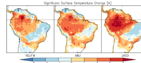
As can be seen in Fig. 4, in the initially dense forest region there is an increase in surface temperature in all seasons; the majority of the region warms by 1–3 K, with the central region warming by more than 7 K. To the southeast, there is a region of temperature decrease, typically less than 3 K. This temperature decrease is largely over the region that was predominantly C4 grass. McGuffie et al. (1995) noted that changes in surface temperature over the deforested region are dipolar: an increase over the central and eastern Amazon and

Figure 4. Change in surface temperature (K) for NDJFM, AMJ and

JASO. Shading indicates significance at the 95 % confidence level.

a decrease to the southwest of the deforestation. The region of decrease is shifted eastward in these findings, but such a dipolar change has a precedent. Additionally, Lorenz and Pitman (2014) note a dipolar temperature change with a de-crease in the east and an inde-crease towards the west, which is noted as being directly related to the initial land–atmosphere coupling strength. Despite the region of cooling, the areal av-erage for each season shows an increase:+0.8 K in NDJFM,

+1.6 K in AMJ, and+2.1 K in JASO.

The contrast in temperature change between the densely forested and C4 grass areas becomes more apparent in the change in maximum monthly surface temperature. The forested region experiences an increase in all months, typi-cally between 2 and 6 K. In the C4 grass area, the maximum monthly surface temperature decreases from August to Jan-uary by 4–6 K, with the remaining months having a mixed change between −2 and 2 K. The same pattern tends to hold up for minimum monthly temperature, with the changes about half the magnitude. The overall range in extremes for the densely forested area increases by 2–4 K, while in the C4 grass area, the range of extremes is reduced by 2–4 K from August to January and increases by less than 2 K in the re-maining months. It is worth noting that C4 grass in CLM can behave unrealistically at times by dying off and then regrow-ing a couple months later (Dirmeyer et al., 2013), which can affect surface temperature drastically.

The annual areal average increase in surface temperature of 1.4 K is consistent with previous modeling studies; Costa and Foley (2000) found a 1.4 K increase, Snyder et al. (2004) found a 1.5 K increase and Snyder (2010) found a 1.2 K in-crease. However, some studies found smaller or larger tem-perature increases: 0.6 K (Henderson-Sellers et al., 1993), 0.3 K (McGuffie et al., 1995), 0.3 K (Ramos da Silva et al., 2008), 2.5 K (Nobre et al., 1991) and 2.5 K (Shukla et al., 1990). The results in this study lie within the range of previ-ous findings.

3.2 Precipitation

Figure 5. Change in precipitation (mm day−1) for NDJFM, AMJ and JASO. Shading indicates significance at the 95 % confidence level.

throughout the year, with some areas experiencing decreases larger than 4 mm day−1; see Fig. 5. The majority of this re-gion sees decreases of more than 50 %. During NDJFM, when the majority of the Amazon region experiences at least 8 mm day−1in precipitation in the control simulation, there is a largely statistically significant decrease in precipitation for the deforested region. An area of increase is present in a region that is mainly irrigated rice. During AMJ when precip-itation is largely occurring within a few degrees of the Equa-tor, there is a significant decrease across this region of the Equator, while a significant increase is present to the south. The driest season in the control simulation, JASO, has a sig-nificant decrease in precipitation over much of the deforested region. All seasons experience a decrease in the areal aver-age:−0.27 mm day−1in NDJFM,−0.37 mm day−1in AMJ, and−0.44 mm day−1in JASO.

Most of the precipitation changes can be explained by changes to convective precipitation, which decreases in all seasons (not shown), with the only exception being the re-gion with irrigated rice. The reduction in convective precipi-tation suggests changes in flux partitioning at the surface may modify the properties and growth of the planetary boundary layer, as well as the land–atmosphere coupling in the region. The decreases exhibited in this study are consistent with previous modeling studies; however, the magnitude of the decrease is smaller. This study found an annual areal av-erage decrease of 0.35 mm day−1, while previous stud-ies found decreases of 0.7 mm day−1 (Costa and Foley, 2000), 0.4–0.7 mm day−1(Hasler et al., 2009), 1.6 mm day−1 (Henderson-Sellers et al., 1993), 1.2 mm day−1 (McGuffie et al., 1995), 1.4 mm day−1 (Snyder et al., 2004; Snyder, 2010), and 0.8 mm day−1 (Werth and Avissar, 2002). The smaller decrease in precipitation may be due to previously mentioned model shortcomings with low humidity and less climatological precipitation in the region.

3.3 Radiation and fluxes

Net radiation is shown (Fig. 6) to be significantly reduced over the densely forest region in all seasons, typically by 30–

Figure 6. Changes in surface energy fluxes in NDJFM, AMJ and

JASO; net radiation (W m−2) (top row), latent heat flux (W m−2) (middle row) and sensible heat flux (W m−2) (bottom row). Shading indicates significance at the 95 % confidence level.

50 W m−2. To the southeast over the C4 grass area, an in-crease is shown during NDJFM, changes between−10 and 10 W m−2_{are present in AMJ, and decreases of 10 W m}−2

exist in JASO. These changes are driven by changes to albedo (seen in Fig. 3) and impacts the partitioning of latent and sen-sible heat flux.

Latent heat flux is primarily reduced across the region in all seasons; the major exception is an increase during ND-JFM in the former C4 grass area. Sensible heat flux increases in the formerly densely forested area in all seasons and is sur-rounded by a region of decrease in sensible heat flux. There is an increase in sensible heat flux in the southeast during both NDJFM and AMJ, while JASO has a mix of both increases and decreases, with most of the area not experiencing a sig-nificant change. The annual areal averages of latent heat flux and sensible heat flux both decrease,−8.1 and−1.7 W m−2, respectively. This change in the fluxes has reduced the evap-orative fraction in the region and indicates that the Amazon would shift to a drier climate.

Figure 7. Changes to evaporative fraction in NDJFM, AMJ and

JASO; shading indicates significance at the 95 % confidence level.

in NDJFM experiences a decrease in evaporative fraction; this is probably due to the deeper root profile of tree PFTs that would have access to a larger soil moisture reservoir.

3.4 Land–atmosphere coupling

A novel aspect of this study is an assessment of the impact on land–atmosphere coupling strength. A two-legged cou-pling metric (Guo et al., 2006; Dirmeyer, 2011) uses corre-lations between a land surface state variable (soil moisture) and surface flux (latent heat) as a means to assess terres-trial climate feedbacks, or a surface flux (sensible heat) and an atmospheric property (PBL height) for the atmospheric climate feedback. It is used here to describe the feedbacks present in the system and how they have changed after defor-estation. Positive values in these two instances would imply that the land surface is controlling the feedback. We multiply these correlations by the standard deviation (SD) of the re-sponse variable (latent heat and PBL height, respectively) to determine the magnitude of the feedback (Guo et al., 2006). The significance of the control simulation coupling strength is based only on the correlation component, and the signifi-cance of the change in coupling strength is based only on the change in correlation (Dirmeyer et al., 2014).

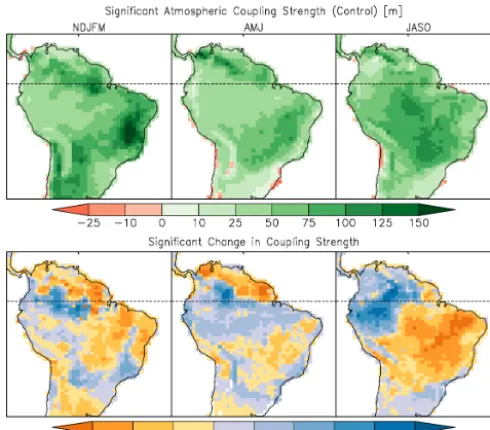
In the terrestrial leg of the coupling (Fig. 8) for the control simulation, a large band of negative values during NDJFM corresponds to the heavy rains during that season when soil moisture is not a limiting factor for surface fluxes. As the rains shift throughout the year, this region shifts accordingly. During the drier seasons in the south, the sign switches to positive, an indication that soil moisture is controlling the latent heat flux (cf. Dirmeyer et al., 2013).

After deforestation, the previously densely forested areas become more strongly coupled throughout the year (Fig. 8). This is probably due to the shallower roots of crops, which have access to a smaller soil moisture reservoir. There are also large areas of decreased coupling, particularly over the southeast in JASO and south of the densely forested area in NDJFM. During AMJ, nearly the whole region sees an in-crease in coupling.

Figure 8. Terrestrial leg of coupling strength (W m−2) between soil moisture and latent heat flux for the control simulation (top row) and change due to deforestation (bottom row) for NDJFM, AMJ and JASO. Shading indicates significance of the correlation component at the 95 % confidence level.

The changes in coupling can occur due to changes in the correlation, variability, or both. In NDJFM, the correlation increases in 54.8 % of the region and flux variability de-creases in 56.4 % of the region. Neither component appears to be the leading agent of the changes; the changes in ND-JFM (the rainy season) are largely atmospherically driven due to changes in precipitation. Areas with the largest re-duction in precipitation have correlation increases; they also have increases in variability and are becoming more strongly coupled.

In AMJ and JASO, the changes in correlation are much larger: 69.5 and 76.6 % of the region have an increase in cor-relation, respectively. Increases in correlation alone do not necessarily imply increased coupling, as the combination of correlation and variance of the fluxes determines coupling strength (Dirmeyer, 2011; Dirmeyer et al., 2012). While the majority of the region in AMJ has stronger coupling, JASO has the majority of the region showing a decrease in cou-pling. JASO has a decrease in variability for 62.7 % of the region, with 46.2 % of the region having an increase in corre-lation and decrease in variability, largely taking place in the southeast, where there was lower initial tree cover. In con-trast, the more densely forested regions largely experience an increase in correlation and an increase in variability.

Figure 9. Atmospheric leg of coupling strength (m) between

sen-sible heat flux and planetary boundary layer height for the control simulation (top row) and change due to deforestation (bottom row) for NDJFM, AMJ and JASO. Shading indicates significance of the correlation component at the 95 % confidence level.

less tree-covered, as the dense canopy acts to dampen the coupling between surface sensible heat flux and PBL height. In all seasons, the densely forested areas have an increase in coupling after deforestation (Fig. 9). The southeastern re-gion largely experiences a decrease in coupling during all seasons. The largest contrast between the densely forested area and the southeast occurs in JASO, which is after most of the crops have been harvested and LAI is low.

For the atmospheric leg, the majority of the region either experiences an increase in both correlation and variability or a decrease in both. There are co-located correlation and variability increases over 31.0, 41.6, and 33.3 % of the gion for NDJFM, AMJ and JASO, respectively. These re-gions are predominantly along the southeastern coast, where increased temperature and decreased precipitation occur, and in the previously forested areas. Regions experiencing de-creases in both were 36.9, 29.7, and 40.2 % for those same seasons. These changes largely occurred in the southeastern area, where lower initial tree cover is located.

4 Discussion and conclusions

Replacement of natural vegetation with crops typical of trop-ical agriculture over the Amazon results in an albedo in-crease, lowering net radiation, which in turn modifies the sur-face fluxes. Latent heat flux is largely reduced across the do-main, with the exception being the former C4 grass region in NDJFM; sensible heat flux has a more detailed spatial change with decreases in all seasons over the former densely forested

Figure 10. Top row: change in the terrestrial leg of coupling

strength (W m−2) versus irrigation water added (mm day−1) for ir-rigated grid boxes in NDJFM, AMJ and JASO. Bottom row: change in the atmospheric leg of coupling strength (m) versus initial tree cover percentage for NDJFM, AMJ and JASO. Shaded dots repre-sent irrigated grid boxes, with the shading being equivalent to the shading for irrigation water added (mm day−1) in the top row.

area and a seasonality to the changes in the surrounding re-gions. The areal averages for latent heat flux and sensible heat flux are reduced, but the evaporative fraction decreases, modifying the region toward a drier climate. Combining the surface temperature increase with the surface flux changes, a warmer, drier and deeper PBL results. There is a decrease in precipitation, largely due to decreased convection, which further alters flux partitioning due to reduced soil moisture. By modifying PBL properties and PBL growth, modified in-teraction between the PBL and the free atmosphere decreases vertical moisture transport and increases vertical heat trans-port. These changes in vertical transport provide a mecha-nism that can impact the circulation and may affect remote regions, with large-scale circulation changes enhancing the precipitation changes.

the less coupled the soil moisture becomes to the latent heat flux.

By affecting the surface coupling, irrigation can also im-pact the atmospheric leg of the coupling (Fig. 10). A negative relationship between irrigation water added and the change in SH-PBLH (atmospheric leg) coupling further shows that irrigation is modifying land–atmosphere interactions.

Although irrigation is shown to have an impact on the atmospheric leg of the coupling, the larger contributor ap-pears to be the percentage of tree cover lost (Fig. 10). The coupling changes are largely the same for non-irrigated grid boxes with original tree percentage less than 80 %, typically between−50 and 50 m. JASO, the driest season, does have a larger spread, but comparable magnitudes of increases and decreases. When the initial tree cover is greater than 80 %, the coupling strength is predominantly increasing and has a greater magnitude of the change. This signal is also com-mon in climate change scenarios driven by greenhouse gas increases (Dirmeyer et al., 2013), suggesting land use change could further amplify sensitivity to land surface anomalies in the tropics.

Irrigation largely decreases the coupling strength when the initial tree cover is less than 80 % and increases the magni-tude of the change. When the initial tree cover is greater than 80 %, the grid boxes that experience a decrease in coupling are typically irrigated, with the more strongly irrigated grid boxes showing the largest decreases and less irrigated grid boxes showing an increase in coupling that is comparable to non-irrigated grid boxes. Just as with the terrestrial leg, more irrigation water added decreases the coupling strength of the atmospheric leg of the coupling.

Even using a realistic heterogeneous crop distribution in the Amazon region, there is still general agreement with pre-vious modeling studies. The higher resolution and hetero-geneity of the land cover show smaller-scale features and regions of opposite change, particularly in the southeastern Amazon, where the region has higher coverage of C4 grass. With crops being planted in different regions at different times of the year, a level of complexity not present in pre-vious Amazon deforestation studies, and seasonality to land surface changes that were not previously modeled, are now seen.

A warming and drying of the region has impacted on how the land surface and atmosphere interact. By modify-ing the flux partitionmodify-ing between latent and sensible heat fluxes, the region shifts to a drier climate with a warmer, drier and deeper PBL. By altering how the PBL grows, in-teraction with the free atmosphere is altered; this can lead to a warmer and drier atmospheric column above the region and may cause impacts to remote regions by modifying the gen-eral circulation and transports of moisture and heat. There is evidence that mesoscale responses of the atmosphere to land surface perturbations at low latitudes may not be well repre-sented in climate models (e.g., Taylor et al., 2013); it would

be worthwhile to repeat tropical deforestation studies with cloud-resolving models in the future.

Remote impacts, such as modification to the African east-erly waves and increased precipitation over the southwestern United States, have been found in these experiments, and will be discussed in a future paper (Badger and Dirmeyer, 2015). By employing a coupled ocean model, changes to sea surface temperature and the El Niño–Southern Oscillation have also been found and will be discussed in a later paper.

Acknowledgements. This research was supported by joint fund-ing from the National Science Foundation (ATM-0830068), the National Oceanic and Atmospheric Administration (NA09OAR4310058), and the National Aeronautics and Space Administration (NNX09AN50G) of the Center for Ocean Land Atmosphere Studies (COLA). The lead author would like to acknowledge Sam Levis (NCAR) for help in getting CLM code modifications and the crop model to work in the coupled CESM, and to NCAR for supplying computing resources on the Yellow-stone supercomputer.

Edited by: P. Gentine

References

Badger, A. M. and Dirmeyer, P. A.: Remote Tropical and Sub-tropical Responses to Amazon Deforestation, Clim. Dynam., 1– 10, doi:10.1007/s00382-015-2752-5, online first, 2015. Bonan, G. B.: Forests and Climate Change: Forcings, Feedbacks,

and the Climate Benefits of Forests, Science, 320, 1444–1449, doi:10.1126/science.1155121, 2008a.

Bonan, G. B.: Ecological Climatology: Concepts and Applications, 2nd Edn., Cambridge University Press, New York, USA, 2008b. Costa, M. H. and Foley, J. A.: Combined Effects of Deforesta-tion and Doubled Atmospheric CO2Concentrations on the Cli-mate of Amazonia, J. CliCli-mate, 13, 18–34, doi:10.1175/1520-0442(2000)013<0018:CEODAD>2.0.CO;2, 2000.

Costa, M. H., Yanagi, S. N. M., Souza, P. J. O. P., Ribeiro, A., and Rocha, E. J. P.: Climate change in Amazonia caused by soybean cropland expansion, as compared to caused by pastureland expansion, Geophys. Res. Lett., 34, L07706, doi:10.1029/2007GL029271, 2007.

Dickinson, R. E. and Henderson-Sellers, A.: Modelling tropical de-forestation: A study of GCM land-surface parametrizations, Q. J. Roy. Meteor. Soc., 114, 439–462, doi:10.1002/qj.49711448009, 1988.

Dirmeyer, P. A.: The terrestrial segment of soil moisture– climate coupling, Geophys. Res. Lett., 38, L16702, doi:10.1029/2011GL048268, 2011.

Dirmeyer, P. A., Cash, B. A., Kinter, J. L., Stan, C., Jung, T., Marx, L., Towers, P., Wedi, N., Adams, J. M., Altshuler, E. L., Huang, B., Jin, E. K., and Manganello, J.: Evidence for Enhanced Land– Atmosphere Feedback in a Warming Climate, J. Hydrometeorol., 13, 981–995, doi:10.1175/JHM-D-11-0104.1, 2012.

Dirmeyer, P. A., Wang, Z., Mbuh, M. J., and Norton, H. E.: Intensified land surface control on boundary layer growth in a changing climate, Geophys. Res. Lett., 41, 1290–1294, doi:10.1002/2013GL058826, 2014.

FAO: available at: http://ecocrop.fao.org, last access: May 2015, 2007.

Foley, J. A., DeFries, R., Asner, G. P., Barford, C., Bonan, G., Car-penter, S. R., Chapin, F. S., Coe, M. T., Daily, G. C., Gibbs, H. K., Helkowski, J. H., Holloway, T., Howard, E. A., Kucharik, C. J., Monfreda, C., Patz, J. A., Prentice, I. C., Ramankutty, N., and Snyder, P. K.: Global Consequences of Land Use, Science, 309, 570–574, doi:10.1126/science.1111772, 2005.

Guo, Z., Dirmeyer, P. A., Koster, R. D., Sud, Y. C., Bonan, G., Ole-son, K. W., Chan, E., Verseghy, D., Cox, P., Gordon, C. T., Mc-Gregor, J. L., Kanae, S., Kowalczyk, E., Lawrence, D., Liu, P., Mocko, D., Lu, C.-H., Mitchell, K., Malyshev, S., McAvaney, B., Oki, T., Yamada, T., Pitman, A., Taylor, C. M., Vasic, R., and Xue, Y.: GLACE: The Global Land–Atmosphere Coupling Experiment. Part II: Analysis, J. Hydrometeorol., 7, 611–625, doi:10.1175/JHM511.1, 2006.

Hasler, N., Werth, D., and Avissar, R.: Effects of Tropical Defor-estation on Global Hydroclimate: A Multimodel Ensemble Anal-ysis, J. Climate, 22, 1124–1141, doi:10.1175/2008JCLI2157.1, 2009.

Henderson-Sellers, A., Dickinson, R. E., Durbidge, T. B., Kennedy, P. J., McGuffie, K., and Pitman, A. J.: Tropical deforestation: Modeling local- to regional-scale climate change, J. Geophys. Res., 98, 7289–7315, doi:10.1029/92JD02830, 1993.

IBGE: Censo Agropecuário 2006, Insituto Brasileiro de Geografia e Estatística, Rio de Janeiro, Brazil, Tech. rep., 311.213.1: 63, 2006.

INPE: PRODES – Amazon deforestation database, INPE, São Jose dos Campos, Tech. rep., 2014.

Kucharik, C. J., Foley, J. A., Delire, C., Fisher, V. A., Coe, M. T., Lenters, J. D., Young-Molling, C., Ramankutty, N., Norman, J. M., and Gower, S. T.: Testing the performance of a dynamic global ecosystem model: water balance, carbon balance, and veg-etation structure, Global Biogeochem. Cy., 14, 795–825, 2000. Lejeune, Q., Davin, E. L., Guillod, B. P., and Seneviratne, S. I.:

In-fluence of Amazonian deforestation on the future evolution of regional surface fluxes, circulation, surface temperature and pre-cipitation, Clim. Dynam., 44, 2769–2786, 2014.

Levis, S., Bonan, G. B., Kluzek, E., Thornton, P. E., Jones, A., Sacks, W. J., and Kucharik, C. J.: Interactive Crop Manage-ment in the Community Earth System Model (CESM1): Seasonal Influences on Land–Atmosphere Fluxes, J. Climate, 25, 4839– 4859, doi:10.1175/JCLI-D-11-00446.1, 2012.

Lorenz, R. and Pitman, A. J.: Effect of land–atmosphere coupling strength on impacts from Amazonian deforestation, Geophys. Res. Lett., 41, 5987–5995, doi:10.1002/2014GL061017, 2014. McGuffie, K., Henderson-Sellers, A., Zhang, H., Durbidge, T.,

and Pitman, A.: Global climate sensitivity to tropical defor-estation, Global Planet. Change, 10, 97–128, doi:10.1016/0921-8181(94)00022-6, 1995.

Nepstad, D. C., Stickler, C. M., Filho, B. S., and Merry, F.: Inter-actions among Amazon land use, forests and climate: prospects for a near-term forest tipping point, Philos. T. R. Soc. B, 363, 1737–1746, doi:10.1098/rstb.2007.0036, 2008.

Nobre, C. A., Sellers, P. J., and Shukla, J.: Amazonian Defor-estation and Regional Climate Change, J. Climate, 4, 957–988, doi:10.1175/1520-0442(1991)004<0957:ADARCC>2.0.CO;2, 1991.

Nobre, P., Malagutti, M., Urbano, D. F., de Almeida, R. A. F., and Giarolla, E.: Amazon Deforestation and Climate Change in a Coupled Model Simulation, J. Climate, 22, 5686–5697, doi:10.1175/2009JCLI2757.1, 2009.

Oleson, K. W., Lawrence, D. M., Bonan, G. B., Drewniak, B., Huang, M., Koven, C. D., Levis, S., Li, F., Riley, W. J., Subin, Z. M., Swenson, S. C., Thornton, P. E., Bozbiyik, A., Fisher, R., Kluzek, E., Lamarque, J.-F., Lawrence, P. J., Leung, L. R., Lipscomb, W., Muszala, S., Ricciuto, D. M., Sacks, W., Sun, Y., Tang, J., and Yang, Z.-L.: Technical Description of version 4.5 of the Community Land Model (CLM), National Center for At-mospheric Research, Boulder, CO, USA, NCAR Technical Note, TN-503+STR, 2013.

Portmann, F. T., Siebert, S., and Döll, P.: MIRCA2000 – Global monthly irrigated and rainfed crop areas around the year 2000: A new high-resolution data set for agricultural and hy-drological modeling, Global Biogeochem. Cy., 24, GB1011, doi:10.1029/2008GB003435, 2010.

Qian, T., Dai, A., Trenberth, K. E., and Oleson, K. W.: Simulation of Global Land Surface Conditions from 1948 to 2004. Part I: Forcing Data and Evaluations, J. Hydrometeorol., 7, 953–975, doi:10.1175/JHM540.1, 2006.

Ramos da Silva, R., Werth, D., and Avissar, R.: Regional Impacts of Future Land-Cover Changes on the Amazon Basin Wet-Season Climate, J. Climate, 21, 1153–1170, doi:10.1175/2007JCLI1304.1, 2008.

Sacks, W. J., Deryng, D., Foley, J. A., and Ramankutty, N.: Crop planting dates: an analysis of global patterns, Global Ecol. Biogeogr., 19, 607–620, doi:10.1111/j.1466-8238.2010.00551.x, 2010.

Shukla, J., Nobre, C., and Sellers, P.: Amazon Deforesta-tion and Climate Change, Science, 247, 1322–1325, doi:10.1126/science.247.4948, 1990.

Snyder, P. K., Delire, C., and Foley, J.: Evaluating the influence of different vegetation biomes on the global climate, Clim. Dynam., 23, 279–302, doi:10.1007/s00382-004-0430-0, 2004.

Snyder, P. K.: The Influence of Tropical Deforestation on the North-ern Hemisphere Climate by Atmospheric Teleconnections, Earth Interact., 14, 1–34, doi:10.1175/2010EI280.1, 2010.

Sun, S. and Wang, G.: Diagnosing the equilibrium state of a cou-pled global biosphere-atmosphere model, J. Geophys. Res., 116, D09108, doi:10.1029/2010JD015224, 2011.

Taylor, C. M., Birch, C. E., Parker, D. J., Dixon, N., Guichard, F., Nikulin, G., and Lister, G. M. S.: Modeling soil moisture-precipitation feedback in the Sahel: Importance of spatial scale versus convective parameterization, Geophys. Res. Lett., 40, 6213–6218, doi:10.1002/2013GL058511, 2013.

Vertenstein, M., Bertini, A., Craig, T., Edwards, J., Levy, M., Mai, A., and Schollenberger, J.: CESM User’s Guide, CESM1.2 Re-lease Series User’s Guide, NCAR Technical Note, National Cen-ter for Atmospheric Research, Boulder, CO, USA, 2013. Werth, D. and Avissar, R.: The local and global effects