A contribution to understanding the turbidity behaviour in an Amazon floodplain

www.hydrol-earth-syst-sci.net/14/351/2010/ © Author(s) 2010. This work is distributed under the Creative Commons Attribution 3.0 License.

Earth System

Sciences

A contribution to understanding the turbidity behaviour in an

Amazon floodplain

E. Alcˆantara1, E. Novo1, J. Stech1, J. Lorenzzetti1, C. Barbosa2, A. Assireu1, and A. Souza2,3

1_{Brazilian Institute for Space Research, Remote Sensing Division, P.O. Box 12227-010, S˜ao Jos´e dos Campos, SP, Brazil} 2_{Brazilian Institute for Space Research, Image Processing Division, P.O. Box 12227-010, S˜ao Jos´e dos Campos, SP, Brazil} 3_{ETEP Faculdades, P.O. Box 12242-800, S˜ao Jos´e dos Campos, SP, Brazil}

Received: 29 April 2009 – Published in Hydrol. Earth Syst. Sci. Discuss.: 26 May 2009 Revised: 23 November 2009 – Accepted: 18 January 2010 – Published: 22 February 2010

Abstract. Observations of turbidity provide quantitative

in-formation about water quality. However, the number of avail-able in situ measurements for water quality determination is usually limited in time and space. Here, we present an analy-sis of the temporal and spatial variability of the turbidity of an Amazon floodplain lake using two approaches: (1) wavelet analysis of a turbidity time series measured by an automatic monitoring system, which should be improved/simplified, and (2) turbidity samples measured in different locations and then interpolated using an ordinary Kriging algorithm. The spatial and temporal variability of turbidity are clearly related to the Amazon River flood pulses in the floodplain. When the water level in the floodplain is rising or receding, the exchange between the Amazon River and the floodplain is the major driving force in turbidity variability. At high-water levels, turbidity variability is controlled by Lake Bathymetry. When the water level is low, wind action and Lake Mor-phometry are the main causes of turbidity variability. The combined use of temporal and spatial data shows a good po-tential for better understanding of the turbidity behaviour in a complex aquatic system such as the Amazon floodplain.

1 Introduction

Turbidity is an important optical parameter in hydrological systems. High turbidity levels are associated with low sun-light penetration in the water column, which can impact pho-tosynthesis and visibility, thereby affecting aquatic organ-isms at all levels in the food chain from microscopic algae

Correspondence to: E. Alcˆantara

([email protected])

to fish. Turbidity depends essentially on the amount of sus-pended particulate material in the water column, which can include phytoplankton, eroded and re-suspended sediments, waste discharge, algae growth and urban runoff (Han and Rundquist, 1998; Wetzel, 2001). Furthermore, it is modu-lated by water flow variation. Changes in turbidity can affect both the zooplankton community (De Leo and Ferrari, 1993) and its composition (Wetzel, 2001), which can in turn elim-inate sensitive organisms (Miquelis et al., 1998) and mod-ify zooplankton taxa competition (Wetzel, 2001). Suspended particles scatter and absorb sunlight, resulting in warmer temperatures and lower concentrations of dissolved oxygen in the water column (Kirk, 1983).

The duration and intensity of a turbidity event are also im-portant issues. A short duration of a very high level turbidity event may not be as significant as a lower level situation that lasts longer (Newcombe and Jensen, 1996). Algal turbidity can vary seasonally and with depth in a complex manner as a response to physical, chemical and biological changes in the water body. Meteorological episodes, such as cold fronts and storms, can have a strong impact on the concentration of in-organic and detritus particles from the watershed (Stech and Lorenzzetti, 1992; Tundisi et al., 2004).

Research about water quality of reservoirs and lakes has been based mostly on point station datasets or along track lines obtained during cruises (Jerosch et al., 2006). High quality in situ measurements of water parameters are usu-ally limited and they are particularly critical for time se-ries data and key variables (Zhang et al., 2003; George, 1997; Dekker et al., 2002; Tyler et al., 2006). The detec-tion of trends and sudden changes in the aquatic system is dependent on both the availability of long-term time series of environmental data and their proper analysis (Stech et al., 2006). Wavelet analysis could be used to understand

352 E. Alcˆantara et al.: Turbidity behaviour in an Amazon floodplain

(a)

4

(a)

(b)

(c)

Figure 1: (a) Location of the Legal Amazon region in Brazil, (b) Legal Amazon limits,

and (c) Location of the Curuai Floodplain (red square in b) and location of the

automatic environmental data collection buoy system SIMA at ‘Lago Grande’. The

arrows indicate the main channels of connection of the Amazon River floodplain.

The water circulation in the floodplain from the beginning of December to the end

January is from west to east (Barbosa, 2005; Barroux, 2006). The main flow channels

from the Amazon River to the Curuai floodplain are located at `Lago Grande`, Lake

`Salé`, and Lake `Santa Ninha` (see Figure 1c).

The average total annual precipitation in the Curuai floodplain is 2447 mm year

,

which is much larger than the average potential evaporation of 1400 mm year

(average

obtained by a time series from 1990 to 2001), with the wet season lasting from January

4

(a)

(b)

(c)

Figure 1: (a) Location of the Legal Amazon region in Brazil, (b) Legal Amazon limits,

and (c) Location of the Curuai Floodplain (red square in b) and location of the

automatic environmental data collection buoy system SIMA at ‘Lago Grande’. The

arrows indicate the main channels of connection of the Amazon River floodplain.

The water circulation in the floodplain from the beginning of December to the end

January is from west to east (Barbosa, 2005; Barroux, 2006). The main flow channels

from the Amazon River to the Curuai floodplain are located at `Lago Grande`, Lake

`Salé`, and Lake `Santa Ninha` (see Figure 1c).

The average total annual precipitation in the Curuai floodplain is 2447 mm year

,

which is much larger than the average potential evaporation of 1400 mm year

(average

obtained by a time series from 1990 to 2001), with the wet season lasting from January

(c)

4

(a)

(b)

(c)

Figure 1: (a) Location of the Legal Amazon region in Brazil, (b) Legal Amazon limits,

and (c) Location of the Curuai Floodplain (red square in b) and location of the

automatic environmental data collection buoy system SIMA at ‘Lago Grande’. The

arrows indicate the main channels of connection of the Amazon River floodplain.

The water circulation in the floodplain from the beginning of December to the end

January is from west to east (Barbosa, 2005; Barroux, 2006). The main flow channels

from the Amazon River to the Curuai floodplain are located at `Lago Grande`, Lake

`Salé`, and Lake `Santa Ninha` (see Figure 1c).

The average total annual precipitation in the Curuai floodplain is 2447 mm year

,

which is much larger than the average potential evaporation of 1400 mm year

(average

obtained by a time series from 1990 to 2001), with the wet season lasting from January

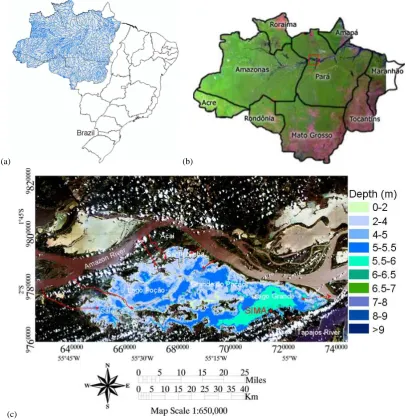
Fig. 1. (a) Location of the Legal Amazon region in Brazil, (b) Legal Amazon limits, and (c) Location of the Curuai Floodplain (red square in

b) and location of the automatic environmental data collection buoy system SIMA at “Lago Grande”. The arrows indicate the main channels of connection of the Amazon River floodplain.

the time-localized frequency content of the signals (Mey-ers et al., 1993; Kumar and Foufoula-Georgiou, 1997) but, on the other hand, the spatial variability patterns could be assessed through geostatistical analysis (Bellehumeur et al., 2000; Hedger et al., 2001).

Here, we show that the combination of a high-resolution time series and spatial data allows for a better understand-ing of the turbidity dynamics in the Amazon floodplain. The main objectives of this paper are to map the spatial distribu-tion patterns of Curua´ı floodplain turbidity along its hydro-logical cycle and to identify the controlling factors in time variability.

2 Study site and background

The Curuai floodplain (Fig. 1) covers an area varying from 1340 to 2000 km2at the low and high-water levels, respec-tively, with a maximum volume reaching 9.3 km3(Martinez and Le-Toan, 2006). This floodplain located 850 km from the Atlantic Ocean, near the city of ´Obidos (Par´a State, Brazil).

The Curua´ı floodplain lakes are interconnected with each other and also to the Amazon River. The Curuai floodplain is controlled by the Amazon River flood pulses, which creates four water-level stages in the floodplain-river system. Water storage in the floodplain starts between November and Jan-uary and lasts until May–June. The drainage phase starts in July and lasts until November. The largest exported volume

occurs from August to October. On an annual basis, the floodplain represents a net source of water to the Amazon River (Bonnet et al., 2008).

During the 2001–2002 water cycle (Bonnet et al., 2008), it was observed that the Amazon River dominated the mixture in early January (64%). From this date until the beginning of April, the river water contribution slightly decreased while contributions from watersheds and direct rainfall increased. By mid-April, the rainfall water constituted as much as 17%. Contributions from the local upland watershed (14%) and from the watershed located in the aquatic-terrestrial transi-tion zone (15%) reached their maximum by the end of Febru-ary. The groundwater reservoir contribution was highest at the end of December, reaching 5% of the mixture.

The water circulation in the floodplain from the beginning of December to the end January is from west to east (Bar-bosa, 2005; Barroux, 2006). The main flow channels from the Amazon River to the Curuai floodplain are located at “Lago Grande”, Lake “Sal´e”, and Lake “Santa Ninha” (see Fig. 1c).

The average total annual precipitation in the Curuai flood-plain is 2447 mm year−1, which is much larger than the av-erage potential evaporation of 1400 mm year−1(average ob-tained by a time series from 1990 to 2001), with the wet season lasting from January to June and a drier season from July to December, resulting in a clear seasonal cycle con-trolling the water level dynamics in the floodplain (Barroux, 2006). The residence time of the riverine water within the floodplain is 5±0.8 months, while the residence time of wa-ter from all sources is 3±0.2 months (Bonnet et al., 2008). The lowest and highest absolute water levels recorded at the Curua´ı gauging station during the 1982–2003 period were 3.03 m and 9.61 m, respectively.

3 The data set and methods

3.1 In situ data

3.1.1 Temporal domain

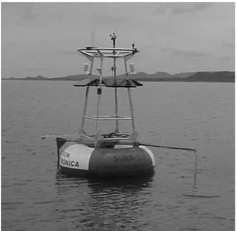
The temporal variability of turbidity in the Curuai floodplain was studied using the data collected by an in-house devel-oped anchored buoy system named Environmental Monitor-ing System – SIMA (Fig. 2). SIMA consists of an anchored buoy and its electronics that are instrumented with a suite of meteorological and water quality sensors (see Fig. 1 for the position of SIMA in Curuai floodplain). The following me-teorological variables were collected: atmospheric pressure, relative humidity, air temperature, wind direction and inten-sity and incoming solar radiation (R. M. Young). The follow-ing water quality parameters were monitored: chlorophyll-a, pH, turbidity, dissolved oxygen, electric conductivity, ni-trate, ammonia and water temperature (YSI multi-parameter probe).

6

Figure 2: Photo of SIMA installed at ‘Lago Grande’ in the Curuai floodplain (See

Figure 1 for location).

Spatial domain

To evaluate the spatial variability of turbidity, several field campaigns of in situ

measurements (using HORIBA U-10 multi-sensor probe) were carried out from 2003 to

2004 at a number of stations (see Figure 3 for locations) and at different Curuai

floodplain lake water levels (Table 1).

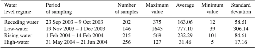
Table 1: Descriptive statistics of the in situ turbidity data (NTU).

Water level

regime

Period of

sampling

Number of

samples

Maximum

value

Average Minimum

value

Standard

deviation

Receding

water

2003/Sep/23

–

2003/Oct/09

202

375

163.06

12

58.61

Low water 2003/Nov/19

-

2003/Dec/01

146

1645

777.10

39

306.14

Rising

water

2004/Feb/01

-

2004/Feb/14

215

569

232.29

101

84.61

High water 2004/May/31

-

2004/Jun/21

256

127

31.46

5

17.16

The HORIBA equipment provides turbidity measurements in NTU (Nephelometric

Turbidity Unit) at a resolution of 1 NTU. A calibration was performed before each day

of sampling. Sampling locations were defined based on the analysis of Landsat-5

Thematic Mapper images acquired at similar floodplain stages (Barbosa, 2005). The

Fig. 2. Photo of SIMA installed at “Lago Grande” in the Curuai

floodplain (See Fig. 1 for location).

The SIMA data were collected in preprogrammed time intervals (1 h) and transmitted via satellite link in quasi-realtime to any user in a range of 2500 km from the acqui-sition point. In this work, we analysed the time series of hourly measurements of turbidity from 20 November 2004 to 26 April 2005. The water depth at the SIMA location was approximately 5.5 m at the high-water level and 1.4 m during the low-water level.

3.1.2 Spatial domain

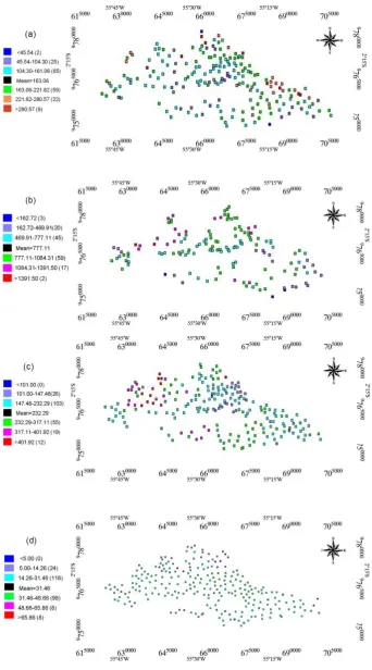
To evaluate the spatial variability of turbidity, several field campaigns of in situ measurements (using HORIBA U-10 multi-sensor probe) were carried out from 2003 to 2004 at a number of stations (see Fig. 3 for locations) and at different Curuai floodplain lake water levels (Table 1).

The HORIBA equipment provides turbidity measurements in NTU (Nephelometric Turbidity Unit) at a resolution of 1 NTU. A calibration was performed before each day of sam-pling. Sampling locations were defined based on the analysis of Landsat-5 Thematic Mapper images acquired at similar floodplain stages (Barbosa, 2005). The periods of data ac-quisition by HORIBA and SIMA were different because the SIMA was installed at the end of 2004. The spatial distri-butions of turbidity samples (statistics presented in Table 1) throughout the Curuai floodplain (in standard deviation bins) are shown in Fig. 3.

354 E. Alcˆantara et al.: Turbidity behaviour in an Amazon floodplain

7 periods of data acquisition by HORIBA and SIMA were different because the SIMA was installed at the end of 2004. The spatial distributions of turbidity samples (statistics presented in Table 1) throughout the Curuai floodplain (in standard deviation bins) are shown in Figure 3.

8

Figure 3: Turbidity samples’ distribution grouped by standard deviation bins (the

numbers between parenthesis indicate the amount of samples that possess one clustering standard deviation): (a) receding water level, (b) low water level, (c) rising water level and (d) high water level.

3.2 Methodological approach

Time series analysis

To analyze the temporal modes of variability of the turbidity time series we used the Fourier Power Spectrum, Wavelet Analysis and Cross Wavelet and Coherence and Phase.

Spectrum analysis deals with the identification of cyclical patterns in the data. Data windowing was used to smooth the power spectrum, thereby reducing its variance, and increasing statistical confidence also may cause spectral leakage (Press et al. 1992). To

Fig. 3. Turbidity samples’ distribution grouped by standard deviation bins (the numbers between parenthesis indicate the amount of samples

that possess one clustering standard deviation): (a) receding water level, (b) low-water level, (c) rising water level and (d) high-water level.

Table 1. Descriptive statistics of the in situ turbidity data (NTU).

Water Period Number Maximum Average Minimum Standard

level regime of sampling of samples value value deviation

Receding water 23 Sep 2003 – 9 Oct 2003 202 375 163.06 12 58.61

Low-water 19 Nov 2003 – 1 Dec 2003 146 1645 777.10 39 306.14

Rising water 1 Feb 2004 – 14 Feb 2004 215 569 232.29 101 84.61

High-water 31 May 2004 – 21 Jun 2004 256 127 31.46 5 17.16

3.2 Methodological approach

3.2.1 Time series analysis

To analyze the temporal modes of variability of the turbidity time series, we used the Fourier Power Spectrum, Wavelet Analysis and Cross Wavelet and Coherence and Phase.

Spectrum analysis deals with the identification of cyclical patterns in the data. Data windowing was used to smooth the power spectrum, thereby reducing its variance and increasing statistical confidence also may cause spectral leakage (Press et al., 1992). To reach a compromise between strong ing (more confidence but stronger bias) and weak smooth-ing (less confidence but less bias) with an acceptable spectral leakage, we generated our power spectrum estimates using a smoothing Hamming window of variable length (Press et al., 1992).

The temporal variability of the frequency content of the turbidity time series was analysed using the Wavelet Trans-form (Meyers et al., 1993; Kumar and Foufoula-Georgiou, 1997; Massei et al., 2006). The decomposing an environ-mental time series into time-frequency space allows for the determination of both the dominant modes of variability and how those modes vary in time. The turbidity time series obtained from SIMA were analysed by continuous wavelet analysis using the Morlet wavelet as the so-called “mother wavelet”.

To get a more detailed view of the importance of the wind on turbidity, which was evidenced by Alcˆantara et al. (2008, 2009), we applied here the cross wavelet and wavelet coher-ence methods in these two time series (Maraun and Kurths, 2004). The cross wavelet transformWxy of the two time seriesxn andyn is a complex function. The cross wavelet power spectrum is defined as|Wxy|, and its complex argu-ment arg (Wxy) can be interpreted as the local relative phase betweenxn andyn in the time-frequency space (Grinsted et al., 2004).

The hourly high-frequency turbidity time series allowed the study of bottom resuspension episodes that cause tur-bidity increases. Particularly in shallow lakes, the effects of wind inducing sediment resuspension have been shown (Booth et al., 2000). These wind-induced physical processes are important for sediment transport and can be dominant

(Lou et al., 2000). We applied the method of Booth et al. (2000) for predicting the wind-induced bottom resuspen-sion at the SIMA location during the low-water level (from November to December).

Wind speed was measured by SIMA at 3 m above the wa-ter surface (Fig. 2). Correction to the standard 10-m height was made using Justus and Mikhail (1976):

U10=Uz _z

za n

, (1)

whereU10 is the wind velocity (ms−1)at 10 m height, Uz is the wind velocity measured by SIMA at heightz, za is the height where the anemometer measures the wind velocity (3 m) andnis given by:

n=

"

0.37−0.088lnUz 1−0.088ln za₁₀

#

. (2)

Wind shear at the surface of the lake transfers energy and momentum to the water column, generating the mean cir-culation, surface and internal waves and turbulence, all of which can lead to vertical mixing (Stevens and Imberger, 1996). The minimum wind velocity needed to generate wave action that reaches the bottom and re-suspends sedi-ment (critical windspeed, Uc) was calculated according to Booth et al. (2000):

Uc=1.2 (

4127 T 3

c F

!)0.813

, (3)

whereUcis the critical wind speed (in ms−1),Tcis the criti-cal wave period andF is the effective fetch (in m) calculated according to Carper and Bachmann (1984).

The basic assumption of this simple model is that the effect of waves is felt down to a depth of approximately L₂, where Lis the wavelength of the surface waves. So, if the water depth (d) is less thanL₂, there is a wave energy transfer to the bottom sediments that can result in sediment resuspension.

The critical wave period (Tc)is given by (CERC, 1984):

Tc= _{4π d}

g 1₂

. (4)

356 E. Alcˆantara et al.: Turbidity behaviour in an Amazon floodplain

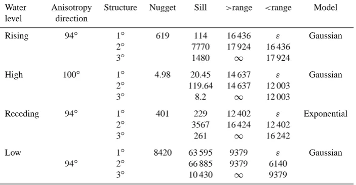
Table 2. Semivariogram parameters used to interpolate the turbidity.

Water Anisotropy Structure Nugget Sill >range <range Model level direction

Rising 94◦ 1◦ 619 114 16 436 ε Gaussian

2◦ 7770 17 924 16 436

3◦ 1480 ∞ 17 924

High 100◦ 1◦ 4.98 20.45 14 637 ε Gaussian

2◦ 119.64 14 637 12 003

3◦ 8.2 ∞ 12 003

Receding 94◦ 1◦ 401 229 12 402 ε Exponential

2◦ 3567 16 424 12 402

3◦ 261 ∞ 16 242

Low 1◦ 8420 63 595 9379 ε Gaussian

94◦ 2◦ 66 885 9379 6140

3◦ 10 430 ∞ 9379

3.2.2 Spatial analysis

Geostatistics is focused on the spatial context and relation-ships present in the data. It provides tools for the quantifi-cation and exploitation of spatial autocorrelation, as well as algorithms for data interpolation with uncertainty quantifi-cation (Isaaks and Srivastava, 1989; Goovaerts, 1997). The autocorrelation structure is used here to estimate the values of variables at points not sampled in the field (Bellehumeur et al., 2000).

A central aspect of geostatistics is the use of spa-tial autocovariance structures, often represented by the (semi)variogram or its cousin, the autocovariogram, which differentiates different kinds of spatial variability (Burrough, 2001). To interpolate in situ turbidity point measurements into a continuous turbidity map, we used the ordinary Krig-ing algorithm. The calculation of the KrigKrig-ing weights was made based upon the semivariogram model.

A fitting of the semivariogram was done using several the-oretical models (spherical, exponential, Gaussian, linear and power) and the weighted least-square method. The theoreti-cal model with minimum standard error was chosen for fur-ther analysis.

Theoretical semivariogram models employ three main co-efficients scaling the fit to the experimental semivariograms: (i) range corresponds to the maximum distance of spatial dependence; (ii) nugget effect is the y-intercept height and corresponds to a random and non-spatially correlated resid-ual variation at the shortest sampling interval; (iii) sill is the height of the curve above its y-intercept (nugget) and cor-responds to the variance due to spatial structure (Isaaks and Srivastava, 1989).

Semivariogram models often have different ranges and/or sills in different directions. For the case where only the range changes with direction, the anisotropy is known as

geometric anisotropy. If only the sill changes with direction, the anisotropy is known as zonal anisotropy. The anisotropy modelling (Isaaks and Srivastava, 1989) usually starts by finding the anisotropy axes associated with the experimen-tally determined directions of minimum and maximum range or sill. The parameters used to interpolate the turbidity sam-ples for each water-level stage are summarized in Table 2.

The equations representing the fitting models used to in-terpolate the turbidity distribution during rising (Eq. 5), high (Eq. 6), receding (Eq. 7) and low (Eq. 8) water levels are:

γ (h)

=619+114[Gau( s

_h 94◦

ε 2

+

_h 216◦

16436 2

)]

+7770[Gau( s

h94◦

17924 2

+

h216◦

16436 2

)]

+1480[Gau( s

_h

94◦

17924 2

+

_h 216◦

∞

2

)] (5)

γ (h)

=4.98+20.45[Gau( s

_h 100◦

ε 2

+

_h 233◦

14637 2

)]

+119.64[Gau( s

_h 100◦

12003 2

+

_h

233◦

14637 2

)]

+8.2[Gau( s

_h

100◦

12003 2

+

_h 233◦

∞

2

)] (6)

γ (h)

=401+229[Exp( s

_h 94◦

ε 2

+

_h 216◦

12402 2

)]

+3567[Exp( s

h94◦

16424 2

+

h216◦

12402 2

)]

+261[Exp( s

_h

94◦

16424 2

+

_h 216◦

∞

2

)] (7)

γ (h)

=8420+7140[Gau( s

_h 94◦

ε 2

+

_h 216◦

6140 2

)]

+66885[Gau( s

_h 94◦

9379 2

+

_h 216◦

6140 2

)]

+10430[Gau( s

_h 94◦

9379 2

+

_h 216◦

∞

2

)] (8)

whereγ (h)is the semivariance at lagh,hn◦ is the

semivari-ance due to angles of anisotropy andε is the range for the lower anisotropy angle. Gau and Exp are the Gaussian and Exponential models, respectively.

4 Results and discussion

4.1 Time series analysis

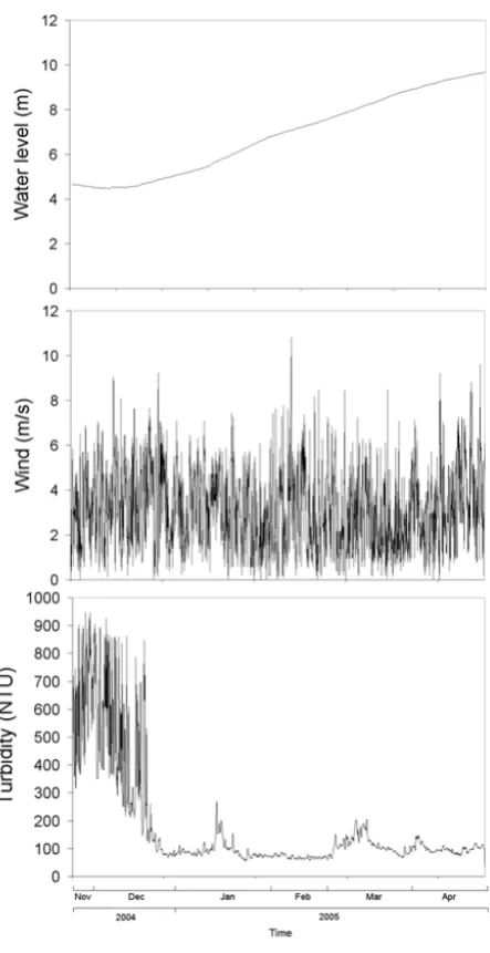
Figure 4 shows the time series plot of water level, wind in-tensity and turbidity. The water level for the studied pe-riod shows minimum, mean and maximum values of 4.45, 6.68 and 9.72 m, respectively. The wind intensity time se-ries has minimum, mean and maximum values of 0, 3.16 and 10.78 ms−1, respectively. The turbidity time series showed a standard deviation of±176.5 NTU with minimum, mean and maximum values of 33.67, 175.28 and 947 NTU, respectively.

The highest values of turbidity were observed from November to the first half of December (2004). From the second half of December to April (2005) the turbidity was relatively small, showing a slowly decreasing trend. Turbid-ity peaks were also observed during this period of low turbid-ity. The smallest values occurred from March to April 2005. The variability of the turbidity timef (t )can be modelled by the following eight-term Gaussian series:

14 Figure 4: Time series of water level (m), wind intensity (ms-1) and turbidity (NTU).

The variability of the turbidity time f(t) can be modeled by the following eight-term

Gaussian series:

Fig. 4. Time series of water level (m), wind intensity (ms−1)and turbidity (NTU).

f (t )

=hexp −

t−µ σ

2!

+386.6exp −

t−106 44.57

2!

+456exp −

t−187 33.91

2!

−428.2exp −

t−317.9 35.99

2!

+642.3exp −

t−308.7 91.08

2!

+102.4exp −

t−802.5 32.56

2!

+80.17exp −

t−1571 85.59

2!

+87.4exp −

t−1458 22.77

2! (9) where (h) is the amplitude, (t) is time, (µ) is the central or peak position and (σ) is the variance.

358 E. Alcˆantara et al.: Turbidity behaviour in an Amazon floodplain

16

Figure 5: Turbidity time series and Gaussian model using the eight-term series (Eq. 9)

(upper panel). Model residuals (lower panel).

The adjustment of this model to the data can be seen in Figure 5. Although the fitting is reasonably good in the mean, during the high variability period from November to December of 2004 the model fitting did not capture all the variability. This is highlighted in Figure 5-b by the high residuals during this period. From the second half of December to April the fitting works very well. The overall fitting was R²=0.94 (p=0.05 andRMSE=36.2). This pattern of variability will be analyzed by Fourier and wavelet analysis.

In general, the turbidity time series shows the response of the Curuai floodplain to the flood pulses (Alcântara, 2006). The highest values of turbidity occurred in the low water level, which may be attributable to sediment resuspension events caused by the waves generated by sufficiently high winds.

The Fourier power spectrum (Figure 6) shows that the highest spectral density occurs from between 90 to 120 hours (3.75 – 5 days). From this point the spectral density falls, and pronounced peaks occur at 80 and 30 hours (3.3 – 1.25 days). The spectral density is very small for frequencies from 0.15 to 0.45 cph-1 _{(6.6 – 2.2 hours).}

Fig. 5. Turbidity time series and Gaussian model using the

eight-term series (Eq. 9) (upper panel). Model residuals (lower panel).

Figure 5 shows the location of all Gaussian terms in Eq. 9. The first Gaussian-term represents the variability of the turbidity in November with a standard deviation (std) of 105.20 (NTU), which was the highest value of the whole series. The second term represents the transition between November and December with a std of 44.57 NTU. The third represents the turbidity variability in the beginning of De-cember (std of 33.91 NTU). The fourth term shows a nega-tive amplitude, representing an abrupt decrease in turbidity values (std of 35.99 NTU). The fifth term shows an increase of turbidity in December, also with an increase of a std to 91.08 NTU. The sixth presents the Gaussian model for the end of December. The seventh and eighth represent the Jan-uary peaks (beginning of the rising water level). Note that from February to April the fitting does not find any other Gaussian term. This is because the turbidity in these months is very low and without great peaks, as opposed to the peaks during November and December (low-water level).

The adjustment of this model to the data can be seen in Fig. 5. Although the fitting is reasonably good in the mean, during the high variability period from November to Decem-ber of 2004 the model fitting did not capture all the variabil-ity. This is highlighted in Fig. 5b by the high residuals dur-ing this period. From the second half of December to April the fitting works very well. The overall fitting wasR2=0.94 (p=0.05 and RMSE=36.2). This pattern of variability will be analysed by Fourier and wavelet analysis.

In general, the turbidity time series shows the response of the Curuai floodplain to the flood pulses (Alcˆantara, 2006). The highest values of turbidity occurred in the low-water level, which may be attributable to sediment resuspension events caused by the waves generated by sufficiently high winds.

17

Figure 6: Fourier power spectrum of the turbidity time series. The dashed lines

represent the 95% confidence interval limits.

All these peaks occur from November (2004) to December (2005). This is due to the high variability of turbidity during this period (Figure 5). For more detail about the localized time frequency, the wavelet analysis is more suitable.

The wavelet analysis shown in Figure 7 reveals that in November 2004 the period of high variability is from 8 to 512 hours (~21 days), while below this the periods are not significant within the 95% confidence level (separated by the cone of influence). Up to December 2004 the periods increase until 2048 hours (~85 days), with peaks in the end of this month between 16-64 hours (~2 days). From January to February 2005 the period increases until 4096 hours (~170 days). From March to April 2005 the periods increase again until 1024 hours (42 days), without periods smaller than 128 hours (~5 days).

In fact the short periods showing in November and December 2004 are due to the high variability of turbidity events. Also, on the other hand, the greater periods from January to April 2005 are due to small variations in turbidity events.

Fig. 6. Fourier power spectrum of the turbidity time series. The

dashed lines represent the 95% confidence interval limits.

The Fourier power spectrum (Fig. 6) shows that the highest spectral density occurs from between 90 to 120 h (3.75–5 days). From this point the spectral density falls, and pronounced peaks occur at 80 and 30 h (3.3–1.25 days). The spectral density is very small for frequencies from 0.15 to 0.45 cph−1(6.6–2.2 h).

All these peaks occur from November (2004) to Decem-ber (2005). This is due to the high variability of turbidity during this period (Fig. 5). For more detail about the local-ized time frequency, the wavelet analysis is more suitable.

The wavelet analysis shown in Fig. 7 reveals that in November 2004 the period of high variability is from 8 to 512 h (∼21 days), while below this the periods are not significant within the 95% confidence level (separated by the cone of influence). Up to December 2004 the peri-ods increase until 2048 h (∼85 days), with peaks in the end of this month between 16–64 h (∼2 days). From January to February 2005 the period increases until 4096 h (∼170 days). From March to April 2005 the periods increase again until 1024 h (42 days), without periods smaller than 128 h (∼5 days).

In fact, the short periods showing in November and De-cember 2004 are due to the high variability of turbidity events. Also, on the other hand, the greater periods from January to April 2005 are due to small variations in turbidity events.

The high mean values and standard deviations of turbid-ity in the low-water level regime are caused mainly by wind action. In the Curuai floodplain, the wind speed can reach 10 ms−1(see Fig. 8). The wind stress induces an energetic wave-affected layer in which both large-scale orbital move-ments and the dissipated turbulent energy are important. The proximity of the surface and bottom boundaries in shallow

18

Figure 7: Wavelet analysis of the turbidity time series. Cross-hatched regions on either

end indicate the “cone of influence,” where edge effects become important.

The high mean values and standard deviations of turbidity in the low water level

regime are caused mainly by wind action. In the Curuai floodplain the wind speed can

reach 10 ms

(see Figure 8). The wind stress induces an energetic wave-affected layer

in which both large-scale orbital movements and the dissipated turbulent energy are

important. The proximity of the surface and bottom boundaries in shallow lakes often

generates a completely mixed water column during the resuspension events (Booth et

al., 2000; Cózar et al., 2005). During the observational period, the winds acquired by

SIMA at ‘Lago Grande’ varied from 0.2 to 10 ms

, with a preferential direction from

southeast to northwest (Figure 8).

Fig. 7. Wavelet analysis of the turbidity time series. Cross-hatched regions on either end indicate the “cone of influence”, where edge effects

become important.

18

Figure 7: Wavelet analysis of the turbidity time series. Cross-hatched regions on either

end indicate the “cone of influence,” where edge effects become important.

The high mean values and standard deviations of turbidity in the low water level regime are caused mainly by wind action. In the Curuai floodplain the wind speed can reach 10 ms-1 _{(see Figure 8). The wind stress induces an energetic wave-affected layer}

in which both large-scale orbital movements and the dissipated turbulent energy are important. The proximity of the surface and bottom boundaries in shallow lakes often generates a completely mixed water column during the resuspension events (Booth et al., 2000; Cózar et al., 2005). During the observational period, the winds acquired by SIMA at ‘Lago Grande’ varied from 0.2 to 10 ms-1, with a preferential direction from southeast to northwest (Figure 8).

Fig. 8. Wind rose diagram of data collected by SIMA from 20 November 2004 to 3 April 2005.

lakes often generates a completely mixed water column dur-ing the resuspension events (Booth et al., 2000; C´ozar et al., 2005). During the observational period, the winds acquired by SIMA at “Lago Grande” varied from 0.2 to 10 ms−1, with a preferential direction from southeast to northwest (Fig. 8). To check the possible causes of sediment resuspension during the low-water level (November, December and Jan-uary), we will apply the critical wave period (CERC, 1984). Our analysis of the suitability of wind to cause resuspension in the high-water level was supported by Novo et al. (2006), who showed a rate less than 0.2 cm h−1of water level change. We checked this for November (2004), event E1, when the variability is larger than that in the other months of the whole time series, as well as for December (2004), event E2, when the variability is smaller than that in November and January (2005), and event E3, where the peaks of variability are more feasibly able to separate due to the rare events of high turbidity.

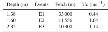
Table 3. Critical wind speed (ms−1) limits to cause bottom sedi-ment resuspension.

Depth (m) Events Fetch (m) Uc (ms−1)

1.38 E1 33 000 0.44

1.60 E2 11 556 1.04

2.32 E3 10 300 1.14

The first event (E1) corresponds to the low-water level, event E2 corresponds to the flow of water from the floodplain to the Amazon River and event E3 takes place when the water level begins to rise in response to the water flowing into the floodplain from the Amazon River.

Events E1, E2 and E3 can probably be attributed to the combination of high wind intensity and shallow-water level. In agreement with Carper and Bachmann (1984), the surface waves produced when wind blows across the surface water cause the bottom resuspension and temporarily increase the turbidity.

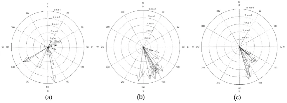
Event E1 has minimum, mean and maximum wind veloc-ities of 0.59, 5.47 and 9.02 ms−1and a preferential wind di-rection from northwest to southeast (Fig. 9a). Event (E2) has minimum, mean and maximum wind velocities of 1.98, 4.5 and 5.75 ms−1_{, with a preferential wind direction from} north-west to southeast, during 24-h (Fig. 9b). Event E3 has mini-mum, mean and maximum wind velocities of 0.34, 2.37 and 5.95 ms−1, with a preferential wind direction from northwest to southeast, during 24-h (Fig. 9c).

The critical wind speed (ms−1)for event E1 is 0.44 and for E2 is 1.04 (Table 3). For event E3 the critical wind speed is 1.14 (ms−1). Wind speeds above these values are suitable for the bottom resuspension in the SIMA location, so both E1 and E2 are suitable for wind-induced bottom resuspension.

360 E. Alcˆantara et al.: Turbidity behaviour in an Amazon floodplain

20

(a)

(b)

(

c)

Figure 9: Compass wind roses of events E1 (a), E2 (b) and E3 (c).

The critical wind speed (ms

) for event E1 is 0.44 and for E2 is 1.04 (Table 3). For

event E3 the critical wind speed is 1.14 (ms

). Wind speeds above these values are

suitable for the bottom resuspension in the SIMA location, so both E1 and E2 are

suitable for wind-induced bottom resuspension.

Table 3: Critical wind speed (ms

) limits to cause bottom sediment resuspension.

Depth (m)

Events

Fetch (m)

Uc (ms

)

1.38

E1

33,000

0.44

1.60

E2

11,556

1.04

2.32

E3

10,300

1.14

20

(a)

(b)

(

c)

Figure 9: Compass wind roses of events E1 (a), E2 (b) and E3 (c).

The critical wind speed (ms

) for event E1 is 0.44 and for E2 is 1.04 (Table 3). For

event E3 the critical wind speed is 1.14 (ms

). Wind speeds above these values are

suitable for the bottom resuspension in the SIMA location, so both E1 and E2 are

suitable for wind-induced bottom resuspension.

Table 3: Critical wind speed (ms

) limits to cause bottom sediment resuspension.

Depth (m)

Events

Fetch (m)

Uc (ms

)

1.38

E1

33,000

0.44

1.60

E2

11,556

1.04

2.32

E3

10,300

1.14

20

(a)

(b)

(

c)

Figure 9: Compass wind roses of events E1 (a), E2 (b) and E3 (c).

The critical wind speed (ms

) for event E1 is 0.44 and for E2 is 1.04 (Table 3). For

event E3 the critical wind speed is 1.14 (ms

). Wind speeds above these values are

suitable for the bottom resuspension in the SIMA location, so both E1 and E2 are

suitable for wind-induced bottom resuspension.

Table 3: Critical wind speed (ms

) limits to cause bottom sediment resuspension.

Depth (m)

Events

Fetch (m)

Uc (ms

)

1.38

E1

33,000

0.44

1.60

E2

11,556

1.04

2.32

E3

10,300

1.14

Fig. 9. Compass wind roses of events E1 (a), E2 (b) and E3 (c).

In Event E1, the peaks of high turbidity and low turbid-ity mark an incidence of unusually low turbidturbid-ity in the low-water level, in spite of the wind speed being above the critical threshold at which sediment resuspension can occur. How-ever, this could be due to the duration of the minimum wind speed (0.59 ms−1)registered by SIMA being low when com-pared with the time series in this water stage. As a conse-quence, a decantation of suspended solids occurs due to the end of the wind action in the surface water.

In accordance with Moreira-Turcq et al. (2004), the silt and clay dominate the suspended solids in the Curuai flood-plain (87–98%), and the decrease of the current velocity oc-curring at the end of wind action causes particle settling. In the low-water stage, the depositional processes in the lakes and channels are disrupted by the wind-induced re-suspension of sediments (Maurice-Bourgoin, 2007) and bio-turbation in shallow lakes (Maia et al., 2008).

To investigate this relationship, we use a cross-wavelet and coherence analysis to register the importance of wind action on turbidity behaviour. Wavelet coherency is a measure of the intensity of the covariance of the two time series in time-frequency space, unlike the cross-wavelet power as a mea-sure of the common power.

4.2 Cross-wavelet spectrum and wavelet coherence

and phase

In Fig. 10a and b, we present the cross-wavelet spectrum and coherency spectrum, respectively. Horizontal arrows indicate a simple linear relationship between turbidity and wind action. Arrows pointing to the right mean correla-tion (in phase), and an anticorrelacorrela-tion (in antiphase) is in-dicated by a left-pointing arrow. Non-horizontal arrows refer to a more complicated (nonlinear) phase difference (Vald´es-Galicia and Velasco, 2008).

The cross wavelet spectrum between the turbidity and wind intensity time series shows a high agreement in the first 500 h (∼20 days, from 20 November 2004 to 10 De-cember 2005) for periods from 4 to 200 h (∼8 days) (see Fig. 10a). These results confirm our findings about the im-portance of the wind action on surface water in enhancing the turbidity during the low-water level.

The coherence is high for this first 500 h, mainly in periods of 4, 8 and 19 h. This coherence in the low time frequency is due to the sediment resuspension caused by wind, as shown in Table 3 (Fig. 10b). The arrows presented in these peri-ods are non-horizontal, representing a complicated, nonlin-ear phase difference.

The agreement between turbidity and wind decreases with rising water levels, in which the wind does not cause as much sediment resuspension. As pointed out by Alcˆantara (2006), in high-water levels the turbidity values are low due to fine sediment decantation. Therefore, the high agreement mi-grates for higher periods (Fig. 10a), following the water level dynamics. Also, the coherence migrates too (Fig. 10b). These influences of wind action and water-level dynamics influence not only the time series domain but also the whole lake.

To investigate the differences in turbidity between the var-ious lakes in the Curuai floodplain, the spatial turbidity dis-tribution over the entire floodplain is determined by applying the ordinary Kriging algorithm on the turbidity collected in situ by a HORIBA U-10 multi-sensor.

4.3 Spatial analysis

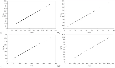
Using a scatterplot, the performance of the ordinary Kriging to interpolate the in situ turbidity data was evaluated for each sampling campaign (Fig. 11). The performance of all inter-polated in situ turbidity data was statistically satisfactory and reliable. The most accurate interpolation was the one made

a

22 (a)

(b)

Figure 10: (a) Cross-wavelet transformation of the standardized turbidity and wind

intensity time series. The 5% significance level against red noise is shown as a thick contour. The relative phase relationship is shown with the arrows. (b) Squared wavelet coherence between the standardized turbidity and wind intensity time series. The 5% significance level against red noise is shown as a thick contour.

The cross wavelet spectrum between the turbidity and wind intensity time series shows a high agreement in the first 500 hours (~20 days, from 20 November 2004 to 10 December 2005) for periods from 4 to 200 hours (~8 days) (see Figure 10-a). These results confirm our findings about the importance of the wind action on surface water in enhancing the turbidity during the low water level.

b

22 (b)

Figure 10: (a) Cross-wavelet transformation of the standardized turbidity and wind

intensity time series. The 5% significance level against red noise is shown as a thick contour. The relative phase relationship is shown with the arrows. (b) Squared wavelet coherence between the standardized turbidity and wind intensity time series. The 5% significance level against red noise is shown as a thick contour.

The cross wavelet spectrum between the turbidity and wind intensity time series shows a high agreement in the first 500 hours (~20 days, from 20 November 2004 to 10 December 2005) for periods from 4 to 200 hours (~8 days) (see Figure 10-a). These results confirm our findings about the importance of the wind action on surface water in enhancing the turbidity during the low water level.

Fig. 10. (a) Cross-wavelet transformation of the standardized turbidity and wind intensity time series. The 5% significance level against red

noise is shown as a thick contour. The relative phase relationship is shown with the arrows. (b) Squared wavelet coherence between the standardized turbidity and wind intensity time series. The 5% significance level against red noise is shown as a thick contour.

(a)

24

(a)

(b)

(c)

(d)

Figure 11: Performance of each interpolated turbidity data: (a) during rising, (b) high,

(c) receding and (d) low water levels.

The semivariogram for the turbidity data during rising, high and low water levels

was best described by a Gaussian model, indicating a smoothly varying pattern in

turbidity distribution. During receding water levels, the semivariogram was best

represented by an exponential function, suggesting a dataset with a spatial pattern

characterized by gradual transition among several patterns interfering with each other

(Burrough and Mcdonnell, 1998) (see Table 2).

In the rising water level regime (Figure 12-a), the flow from the Amazon River to the

Curuai floodplain starts in a channel located at the eastern border of the lake, and then it

migrates to small channels at the northwestern border (Alcântara et al, 2009). The

yellow circle 1 marks a region of high turbidity formed by the water from the Amazon

River entering through the channel located at the eastern border. The region of high

turbidity marked by the yellow circle 2 was formed by water entering through the small

channels located on the northwestern side. The yellow circle 3 marks a region of low

turbidity.

In the high water level regime (Figure 12-b), the input of water from the Amazon

River is lowest, and the turbidity tends to be spatially homogeneous (Alcântara et al.

2008). The areas of high turbidity (marked 1 and 2) correspond to the small channels

connecting the floodplain with the Amazon River. Area 3 also corresponds to a

(b)

24

(a)

(b)

(c)

(d)

Figure 11: Performance of each interpolated turbidity data: (a) during rising, (b) high,

(c) receding and (d) low water levels.

The semivariogram for the turbidity data during rising, high and low water levels

was best described by a Gaussian model, indicating a smoothly varying pattern in

turbidity distribution. During receding water levels, the semivariogram was best

represented by an exponential function, suggesting a dataset with a spatial pattern

characterized by gradual transition among several patterns interfering with each other

(Burrough and Mcdonnell, 1998) (see Table 2).

In the rising water level regime (Figure 12-a), the flow from the Amazon River to the

Curuai floodplain starts in a channel located at the eastern border of the lake, and then it

migrates to small channels at the northwestern border (Alcântara et al, 2009). The

yellow circle 1 marks a region of high turbidity formed by the water from the Amazon

River entering through the channel located at the eastern border. The region of high

turbidity marked by the yellow circle 2 was formed by water entering through the small

channels located on the northwestern side. The yellow circle 3 marks a region of low

turbidity.

In the high water level regime (Figure 12-b), the input of water from the Amazon

River is lowest, and the turbidity tends to be spatially homogeneous (Alcântara et al.

2008). The areas of high turbidity (marked 1 and 2) correspond to the small channels

connecting the floodplain with the Amazon River. Area 3 also corresponds to a

(c)

24

(a)

(b)

(c)

(d)

Figure 11: Performance of each interpolated turbidity data: (a) during rising, (b) high,

(c) receding and (d) low water levels.

The semivariogram for the turbidity data during rising, high and low water levels

was best described by a Gaussian model, indicating a smoothly varying pattern in

turbidity distribution. During receding water levels, the semivariogram was best

represented by an exponential function, suggesting a dataset with a spatial pattern

characterized by gradual transition among several patterns interfering with each other

(Burrough and Mcdonnell, 1998) (see Table 2).

In the rising water level regime (Figure 12-a), the flow from the Amazon River to the

Curuai floodplain starts in a channel located at the eastern border of the lake, and then it

migrates to small channels at the northwestern border (Alcântara et al, 2009). The

yellow circle 1 marks a region of high turbidity formed by the water from the Amazon

River entering through the channel located at the eastern border. The region of high

turbidity marked by the yellow circle 2 was formed by water entering through the small

channels located on the northwestern side. The yellow circle 3 marks a region of low

turbidity.

In the high water level regime (Figure 12-b), the input of water from the Amazon

River is lowest, and the turbidity tends to be spatially homogeneous (Alcântara et al.

2008). The areas of high turbidity (marked 1 and 2) correspond to the small channels

connecting the floodplain with the Amazon River. Area 3 also corresponds to a

(d)

24

(a)

(b)

(c)

(d)

Figure 11: Performance of each interpolated turbidity data: (a) during rising, (b) high,

(c) receding and (d) low water levels.

The semivariogram for the turbidity data during rising, high and low water levels

was best described by a Gaussian model, indicating a smoothly varying pattern in

turbidity distribution. During receding water levels, the semivariogram was best

represented by an exponential function, suggesting a dataset with a spatial pattern

characterized by gradual transition among several patterns interfering with each other

(Burrough and Mcdonnell, 1998) (see Table 2).

In the rising water level regime (Figure 12-a), the flow from the Amazon River to the

Curuai floodplain starts in a channel located at the eastern border of the lake, and then it

migrates to small channels at the northwestern border (Alcântara et al, 2009). The

yellow circle 1 marks a region of high turbidity formed by the water from the Amazon

River entering through the channel located at the eastern border. The region of high

turbidity marked by the yellow circle 2 was formed by water entering through the small

channels located on the northwestern side. The yellow circle 3 marks a region of low

turbidity.

In the high water level regime (Figure 12-b), the input of water from the Amazon

River is lowest, and the turbidity tends to be spatially homogeneous (Alcântara et al.

2008). The areas of high turbidity (marked 1 and 2) correspond to the small channels

connecting the floodplain with the Amazon River. Area 3 also corresponds to a

Fig. 11. Performance of each interpolated turbidity data: (a) during rising, (b) high, (c) receding and (d) low-water levels.

for the data in the high-water level regime (RMSE=3 NTU), while the interpolation for the low-water level regime was the least accurate (RMSE=25 NTU).

This is a result of the water level stability and low stan-dard deviation in the high-water level regime (mean=31.46, see Fig. 3d), as well as the high standard deviation (mean=771.11, see Fig. 3b) and sediment resuspension events in the low-water level regime (see Table 3).

All in situ turbidity data were interpolated using the or-dinary Kriging algorithm to assess the turbidity distribution and variability in response to flood pulses (Fig. 12). Accord-ing to Bonnet et al. (2008), the water storage within the flood-plain started between December and February and lasted un-til June. From this time unun-til the end of the water year, water was exported from the floodplain into the river, with the max-imum water export occurring from August to September.

362 E. Alcˆantara et al.: Turbidity behaviour in an Amazon floodplain

26

Figure 12: Ordinary Kriging maps: (a) turbidity distribution (NTU) during rising, (b)

high, (c) receding and (d) low water levels.

Conclusions

This result shows the importance of high-frequency and spatial data in limnological studies of complex aquatic systems (i.e., the Amazon floodplain), in contrast to

Fig. 12. Ordinary Kriging maps: (a) turbidity distribution (NTU)

during rising, (b) high, (c) receding and (d) low-water levels.

The semivariogram for the turbidity data during rising, high- and low-water levels was best described by a Gaussian model, indicating a smoothly varying pattern in turbidity dis-tribution. During receding water levels, the semivariogram was best represented by an exponential function, suggest-ing a dataset with a spatial pattern characterised by gradual transition among several patterns interfering with each other (Burrough and Mcdonnell, 1998) (see Table 2).

In the rising water level regime (Fig. 12a), the flow from the Amazon River to the Curuai floodplain starts in a channel located at the eastern border of the lake, and then it migrates to small channels at the northwestern border (Alcˆantara et al., 2009). The yellow circle 1 marks a region of high tur-bidity formed by the water from the Amazon River entering through the channel located at the eastern border. The region of high turbidity marked by the yellow circle 2 was formed by water entering through the small channels located on the northwestern side. The yellow circle 3 marks a region of low turbidity.

In the high-water level regime (Fig. 12b), the input of wa-ter from the Amazon River is lowest and the turbidity tends to be spatially homogeneous (Alcˆantara et al., 2008). The areas of high turbidity (marked 1 and 2) correspond to the small

channels connecting the floodplain with the Amazon River. Area 3 also corresponds to a connecting channel, however, its turbidity is low. This probably occurs because this channel is the first to cease flowing water into the floodplain. Area 4 has a low turbidity due to the forest cover, favouring a de-crease in flow velocity and particle settling because of lower hydrodynamics.

In the receding water level regime (Fig. 12c), the preferen-tial direction of flow is from west to east (Barbosa, 2005). As a result, the regions marked 1 and 2 in Fig. 12c show a high turbidity due to the friction of water at the channel borders. The high turbidity in area 3 stems from suspended solids en-tering from the east channel connected to the Amazon River. The receding water level stage causes a condition of turbulent flow, thereby leading to increased turbulence.

In the low-water level regime (Fig. 12d), the exchange be-tween the Amazon River and the Curuai floodplain reaches a minimum, and the turbidity variability is mainly wind-driven. As discussed above, the preferential wind direction is from southeast to northwest (Fig. 8), causing water to pile up and generate a dowelling near the channel margins and an up-welling in the opposite direction. These regions are marked by the yellow circles 1 and 2.

5 Conclusions

This result shows the importance of high-frequency and spa-tial data in limnological studies of complex aquatic systems (i.e., the Amazon floodplain), in contrast to conventional studies with only occasional sampling that can lead to the misinterpretation of the turbidity behaviour.

The flood pulse that occurs with the rising waters of the Amazon flood introduces turbidity from 80 to 180 NTU. Dur-ing the low-water period the wind stirs up the bottom sedi-ments, leading to turbidities in excess of 1100 NTU. There-fore, the highest turbidities and the greatest variability are caused by wind blowing over shallow water. The analysis of the spatially distributed turbidity samples with the ordi-nary Kriging algorithm showed the same dependence on wa-ter level and wind observed by SIMA in the time series in a single sampling point.

The Fourier power spectrum reveals peaks of high spectral density from 3.75 to 5 days and small spectral density from 2 to 6.6 h. The wavelet analysis locates this on the time-frequency domain. During low-water levels, the high turbid-ity variabilturbid-ity occurs from 21 to 85 days. However, peaks of 2 days can occur in association with re-suspension events. In rising water levels, these periods rise to 170 days in the be-ginning of the stage, and from the middle to the end the pe-riods of variability are lower (from 5 to 42 days). The cross wavelet analysis confirms the results obtained by the Fourier and Wavelet analysis, showing that, during low-water levels, the high common power occurs for periods less than 2.66 days and the period rises as the water level rises.

The only water level stage lacking simultaneously ac-quired SIMA time series and spatially distributed data was the high-water period. However, the time variability during the high-water period is small due to the inhibition of sedi-ment re-suspension by the weak winds and sedisedi-ment settling. The information on the sediment behaviour of the floodplain during high water was captured by the spatial data analysis.

Spatially distributed and time series limnological data should be viewed as complimentary. The lack of a high temporal resolution time series may result in severe under sampling. For example, quick but important events of re-suspension might be not observed at all. Also, the availabil-ity of ancillary meteorological time series help to elucidate important relationships between sediment concentration and forcing, such as those demonstrated in this paper. On the other hand, spatial maps allow a better view of the patterns of variability throughout the floodplain. This is particularly important in such complex systems as the Curuai. When fea-sible, spatial and temporal data should be used together for more accurate results.

Acknowledgements. The authors are grateful to the Brazilian

funding agency FAPESP under grants 02/09911-1 and the Brazilian Council for Scientific and Technological Development (CNPq) for the M.Sc fellowship to E. H. Alcˆantara. We also thank C. Torrence and G. Compo for providing the Wavelet soft-ware available at http://atoc.colorado.edu/research/wavelets/, as well as A. Gristed for providing the cross-wavelet and wavelet coherence algorithm software available at http://www.pol.ac.uk/home/research/waveletcoherence/.

Edited by: A. Ghadouani

References

Alcˆantara, E. H.: Analysis of turbidity in Curuai floodplain through the integration of telemetric and MODIS/Terra image data (MSc. Dissertation), INPE: S˜ao Jos´e dos Campos, Brazil, 220 pp., 2006 (in Portuguese).

Alcˆantara, E. H., Stech, J. L., Novo, E. M. L. M., Shimabukuro, Y. E., and Barbosa, C. C. F.: Turbidity in the Amazon floodplain as-sessed through a spatial regression model applied to fraction im-ages derived from MODIS/Terra. IEEE Trans. Geo. Rem. Sens. 46, 2895–2905, 2008.

Alcˆantara, E. H., Barbosa, C. C. F., Stech, J. L., Novo, E. M. L. M., and Shimabukuro, Y. E.: Improving the spectral unmixing algorithm to map water turbidity distributions. Environ. Modell. Softw., 24, 1051–1061, 2009.

Barbosa, C. C. F.: Sensoriamento remoto da dinˆamica de circulac¸˜ao da ´agua do sistema plan´ıcie de Curuai/ Rio Amazonas (PhD. The-sis), INPE: S˜ao Jos´e dos Campos, Brazil, 255 pp., 2005. Barroux, G.: Bio-geochemical study of a lake system from the

Amazonian floodplain: the case of “Lago Grande de Curua´ı”, Par´a-Brazil (PhD Thesis), UPS: Toulouse, France , 304 pp., 2006 (in French).

Bellehumeur, C., Marcotte, D., and Legendre, P.: Estimation of re-gionalized phenomena by geostatistical methods: lake acidity on the Canadian Shield, Environ. Geol., 39, 211–220, 2000. Bonnet, M. P., Barroux, G., Martinez, J. M., Seyler, F.,

Moreira-Turcq, P., Cochonneau, G., Melack, J. M., Boaventura, G., Maurice-Bourgoin, L., Le´on, J. G., Roux, E., Calmant, S., Ko-suth, P., Guyot, J. L., and Seyler, P.: Floodplain hydrology in an Amazon floodplain lake (Lago Grande de Curua´ı), J. Hydrol., 349, 18–30, 2008.

Booth, J. G., Miller, R. L., McKee, B. A., and Leathers, R. A.: Wind-induced bottom sediment resuspension in a microtidal coastal environment, Cont. Shelf Res., 20, 785–806, 2000. Burrough, P. A.: GIS and Geostatistics: Essential partners for

spa-tial analysis. Environ. Ecol. Stat. 8, 361–377, 2001.

Burrough, P. A. and Mcdonnell, R. A.: Principles of geographi-cal information systems, 2rd Ed., Oxford University Press, New York, USA, 356 pp., 1998.

Carper, G. L. and Bachmann, R. W.: Wind resuspension of sedi-ments in a prairie lake, Can. J. Fish. Aquat. Sci. 41, 1763–1767, 1984.

CERC: Shore protection manual, 1rd Ed, US Army Coastal Engi-neering Center, Viksburg, USA, 603 pp., 1984.

C´ozar, A., G´alvez, J. A., Hull, V., Garc´ıa, C. M., and Loiselle, S. A.: Sediment resuspension by Wind in a shallow lake of Esteros Del Iber´a (Argentina): a model based on turbidimetry, Ecol. Model. 186, 63–76, 2005.

De Leo, G. A. and Ferrari, I.: Disturbance and diversity in a river zooplankton community: a neutral model analysis, Coenoses., 8, 121–129, 1993.

Dekker, A. G., Vos, R. J., and Peters, S. W. M.: Analytical algo-rithms for lake water TSM estimation for retrospective analyses of TM and SPOT sensor data, Int. J. Remote Sens. 23, 15–35, 2002.

Farge, M.: Wavelet transforms and their applications to turbulence, Annu. Rev. Fluid Mech. 24, 395–457, 1992.

George, D. G.: The airborne remote sensing of phytoplankton chlorophyll in the lakes and tarns of the English Lake District, Int. J. Remote Sens. 18, 1961–1975, 1997.

Goovaerts, P.: Geostatistics for natural resources evaluation, Oxford University Press, New York, USA, 483 pp., 1997.

Grinsted, A., Moore, J. C., and Jevrejeva, S.: Application of the cross wavelet transform and wavelet coherence to geophysical time series, Nonlinaer Proc. Geoph. 11, 561–566, 2004. Han, L. and Rundquist, D. C.: The impact of a wind-roughened

wa-ter surface on remote measurements of turbidity, Int. J. Remote Sens. 19, 195–201, 1998.

Hedger, R. D., Atkinson, P. M., and Malthus, T. J.: Optimizing sam-pling strategies for estimating mean water quality in lakes using geostatistical techniques with remote sensing, Lakes & Reser-voirs, Res. Manage., 6, 279–288, 2001.

Isaaks, E. H. and Srivastava, M. R.: An introduction to applied geostatistics, Oxford University Press, New York, USA, 561 pp., 1989.

Jerosch, K., Schl¨uter, M., and Pesch, R.: Spatial analysis of marine categories information using indicator Kriging applied to georef-erenced video mosaics of the deep-sea H˚akon Mosby Mud Vol-cano, Ecol. Inform., 1, 391–406, 2006.