https://doi.org/10.5194/hess-22-1175-2018 © Author(s) 2018. This work is distributed under the Creative Commons Attribution 3.0 License.
Evaluation of statistical methods for quantifying fractal scaling in
water-quality time series with irregular sampling
Qian Zhang1, Ciaran J. Harman2, and James W. Kirchner3,4,5
1University of Maryland Center for Environmental Science, US Environmental Protection Agency Chesapeake Bay Program Office, 410 Severn Avenue, Suite 112, Annapolis, Maryland 21403, USA
2Department of Environmental Health and Engineering, Johns Hopkins University, 3400 North Charles Street, Baltimore, Maryland 21218, USA
3Department of Environmental System Sciences, ETH Zurich, Universitätstrasse 16, 8092 Zurich, Switzerland 4Swiss Federal Research Institute WSL, Zürcherstrasse 111, 8903 Birmensdorf, Switzerland
5Department of Earth and Planetary Science, University of California, Berkeley, Berkeley, California 94720, USA Correspondence:Qian Zhang ([email protected])
Received: 30 May 2017 – Discussion started: 21 June 2017
Revised: 21 November 2017 – Accepted: 19 December 2017 – Published: 12 February 2018
Abstract.River water-quality time series often exhibit frac-tal scaling, which here refers to autocorrelation that decays as a power law over some range of scales. Fractal scal-ing presents challenges to the identification of deterministic trends because (1) fractal scaling has the potential to lead to false inference about the statistical significance of trends and (2) the abundance of irregularly spaced data in water-quality monitoring networks complicates efforts to quantify fractal scaling. Traditional methods for estimating fractal scaling – in the form of spectral slope (β) or other equivalent scaling parameters (e.g., Hurst exponent) – are generally inapplica-ble to irregularly sampled data. Here we consider two types of estimation approaches for irregularly sampled data and evaluate their performance using synthetic time series. These time series were generated such that (1) they exhibit a wide range of prescribed fractal scaling behaviors, ranging from white noise (β =0) to Brown noise (β=2) and (2) their sampling gap intervals mimic the sampling irregularity (as quantified by both the skewness and mean of gap-interval lengths) in real water-quality data. The results suggest that none of the existing methods fully account for the effects of sampling irregularity onβestimation. First, the results illus-trate the danger of using interpolation for gap filling when ex-amining autocorrelation, as the interpolation methods consis-tently underestimate or overestimateβunder a wide range of prescribedβvalues and gap distributions. Second, the widely used Lomb–Scargle spectral method also consistently
under-estimatesβ. A previously published modified form, using only the lowest 5 % of the frequencies for spectral slope esti-mation, has very poor precision, although the overall bias is small. Third, a recent wavelet-based method, coupled with an aliasing filter, generally has the smallest bias and root-mean-squared error among all methods for a wide range of pre-scribedβvalues and gap distributions. The aliasing method, however, does not itself account for sampling irregularity, and this introduces some bias in the result. Nonetheless, the wavelet method is recommended for estimatingβin irregular time series until improved methods are developed. Finally, all methods’ performances depend strongly on the sampling irregularity, highlighting that the accuracy and precision of each method are data specific. Accurately quantifying the strength of fractal scaling in irregular water-quality time se-ries remains an unresolved challenge for the hydrologic com-munity and for other disciplines that must grapple with irreg-ular sampling.
1 Introduction
1.1 Autocorrelations in time series
in the past. This property is usually characterized by the au-tocorrelation function (ACF), which is defined as follows for a processXtat lagk:
γ (k)=cov(Xt, Xt+k) . (1)
In practice, autocorrelation has been frequently modeled with classical techniques such as autoregressive (AR) or autore-gressive moving-average (ARMA) models (Darken et al., 2002; Yue et al., 2002; Box et al., 2008). These models as-sume that the underlying process has short-term memory; i.e., the ACF decays exponentially with lag k (Box et al., 2008).
Although the short-term memory assumption holds some-times, it cannot adequately describe many time series whose ACFs decay as a power law (thus much slower than expo-nentially) and may not reach zero even for large lags, which implies that the ACF is non-summable. This property is com-monly referred to as long-term memory or fractal scaling, as opposed to short-term memory (Beran, 2010).
Fractal scaling has been increasingly recognized in stud-ies of hydrological time serstud-ies, particularly for the common task of trend identification. Such hydrological series include river flows (Montanari et al., 2000; Khaliq et al., 2008, 2009; Ehsanzadeh and Adamowski, 2010), air and sea temperatures (Fatichi et al., 2009; Lennartz and Bunde, 2009; Franzke, 2012a, b), conservative tracers (Kirchner et al., 2000, 2001; Godsey et al., 2010), and non-conservative chemical con-stituents (Kirchner and Neal, 2013; Aubert et al., 2014). Be-cause for fractal scaling processes the variance of the sam-ple mean converges to zero much slower than the rate of n−1 (n: sample size), the fractal scaling property must be taken into account to avoid false positives (Type I errors) when inferring the statistical significance of trends (Cohn and Lins, 2005; Fatichi et al., 2009; Ehsanzadeh and Adamowski, 2010; Franzke, 2012a). Unfortunately, as stressed by Cohn and Lins (2005), it is “surprising that nearly every assessment of trend significance in geophysical variables published dur-ing the past few decades has failed [to do so]”, and a similar tendency is evident in the decade following that statement as well.
1.2 Overview of approaches for quantification of fractal scaling
Several equivalent metrics can be used to quantify frac-tal scaling. Here we provide a review of the definitions of such processes and several typical modeling approaches, in-cluding both time-domain and frequency-domain techniques, with special attention to their reconciliation. For a more com-prehensive review, readers are referred to Beran et al. (2013), Boutahar et al. (2007), and Witt and Malamud (2013).
Strictly speaking, Xt is called a stationary long-memory
process if the condition lim
k→∞k
αγ (k)=C
1>0, (2)
whereC1 is a constant and is satisfied by some α∈(0,1) (Boutahar et al., 2007; Beran et al., 2013). Equivalently,Xt
is a long-memory process if, in the spectral domain, the con-dition
lim
ω→0
|ω|βf (ω)=C2>0 (3)
is satisfied by someβ∈(0,1), whereC2is a constant and
f (ω) is the spectral density function of Xt, which is
re-lated to ACF as follows (which is also known as the Wiener– Khinchin theorem):
f (ω)= 1
2π
∞ X
k=−∞
γ (k) e−ikω, (4)
whereωis angular frequency (Boutahar et al., 2007). One popular model for describing long-memory processes is the so-called fractional autoregressive integrated moving-average model, or ARFIMA (p,q,d), which is an extension of ARMA models and is defined as follows:
(1−B)dϕ(B)Xt =ψ (B)εt, (5)
whereεt is a series of independent, identically distributed
Gaussian random numbers (0,σε2),Bis the backshift opera-tor (i.e.,BXt =Xt−1), and functionsϕ(•) andψ(•) are
poly-nomials of orderpandq, respectively. The fractional differ-encing parameterdis related to the parameterαin Eq. (2) as follows:
d=1−α
2 ∈(−0.5,0.5) (6)
(Beran et al., 2013; Witt and Malamud, 2013).
In addition to a slowly decaying ACF, a long-memory pro-cess manifests itself in two other equivalent fashions. One is the so-called Hurst effect, which states that, on a log–log scale, the range of variability of a process changes linearly with the length of the time period under consideration. This power-law slope is often referred to as the Hurst exponent or Hurst coefficientH (Hurst, 1951), which is related tod as follows:
H=d+0.5 (7)
(Beran et al., 2013; Witt and Malamud, 2013).
The second equivalent description of long-memory pro-cesses, this time from a frequency-domain perspective, is fractal scaling, which describes a power-law decrease in spectral power with increasing frequency, yielding power spectra that are linear on log–log axes (Lomb, 1976; Scargle, 1982; Kirchner, 2005). Mathematically, this inverse propor-tionality can be expressed as
f (ω)=C3|ω|−β, (8)
● ● ● ● ● ● ● ●● ● ● ● ●
● ● ●● ●● ● ●● ●
● ● ●● ● ● ● ●
● ● ● ● ●●● ● ● ● ● ●●
● ● ● ● ● ● ● ● ●
● ● ●
● ● ● ● ●
● ● ● ● ●
● ● ● ●
● ● ●
● ● ● ● ●● ●● ● ●
● ● ● ● ● ●● ● ● ● ● ● ●
● ● ● ● ● ● ● ● ● ● ●● ● ●
●● ●
● ●●●●
● ● ● ●
●●● ● ●● ●● ● ● ●
● ●
● ● ● ● ●
● ●
● ● ● ● ●
● ● ● ● ● ● ● ● ● ●
● ● ●
● ● ●●
● ●
● ● ● ● ●
● ● ● ●● ● ● ●●
● ● ●
● ● ● ●
●●● ● ● ● ●
●● ●
● ● ●
0 50 100 150 200
−3
−1
1
3
β = 0 (white noise)
Time step
V
alue
(a) No gap
●●● ● ● ● ● ●● ● ● ● ● ● ● ● ● ●●●●
● ● ● ● ● ● ● ● ● ● ●● ● ● ●● ● ●● ● ● ●● ●● ●●● ● ● ● ● ● ● ●
● ● ●● ● ●● ● ●● ● ● ● ● ● ● ● ● ● ● ●●●●●
● ● ● ●●● ● ●● ● ● ● ●● ● ●● ● ●● ● ● ●● ● ●● ● ● ●● ● ●●●●●
● ●● ● ●●●●●●
●●● ●● ● ● ● ●●●●
● ● ● ●● ● ● ● ●● ●● ● ● ● ● ● ●● ● ● ● ●● ● ● ● ● ● ● ● ●● ●●● ● ● ● ●
● ● ● ● ● ● ● ●● ● ●●● ● ●● ● ● ● ●
0 50 100 150 200
−3
−1
1
3
β = 1 (pink noise)
Time step
V
alue
(b) No gap
●●●●●●●●●●● ● ●● ●●●●●●●●
● ●●●●●●●
●●●●●●●●●●●●●●●●●●● ● ●●●●●
● ●●●●●●●●●●●
●●● ● ● ● ●●●●●●●●●●●●●
●●●●●●●●● ● ● ●●●●●●●●
● ●●●●
●●● ● ●●●●●●●●●●●●●●●●●●●
●● ●●●●●●●●●●●
●● ●●●●●●●
● ●●● ●●●●●●
● ●●●
●●●●●●●●●●● ●●● ●●●●
●●●●●●●●●●●●●
0 50 100 150 200
−3
−1
1
3
β = 2 (Brown noise)
Time step
V
alue
(c) No gap
●● ●● ● ● ● ● ● ●●
● ●● ● ●●
● ● ● ● ● ● ● ● ●●
● ●●
●
● ● ●
● ● ● ● ● ● ● ● ● ●
● ● ● ● ● ● ● ● ●
● ●
● ●●● ● ●●●●
● ● ● ● ●
● ● ●
● ● ● ● ● ●●
● ● ●
● ●
● ●●
● ●
● ●
● ● ● ● ● ● ● ●
●
0 50 100 150 200
−3
−1
1
3
β = 0 (white noise)
Time step
V
alue
(d) Gap: λ = 1, µ = 1
●● ●●
● ●●●
●●●
● ● ● ● ●●
● ● ● ● ●● ●●●●
● ● ● ● ● ●
●●● ●●●●
● ●● ●
● ● ● ● ● ● ● ● ● ● ● ●●●●
● ●●●●
●●● ● ● ● ●
● ● ● ●●●
●● ● ●●
● ● ● ●●
● ●
● ● ● ● ● ● ●●●
● ●
0 50 100 150 200
−3
−1
1
3
β = 1 (pink noise)
Time step
V
alue
(e) Gap: λ = 1, µ = 1
●● ● ●●●●●●●●
●●●●●●● ● ●●●●●●●●●●●
● ● ●
●●●●●●● ● ●● ● ●●●●●
●●●● ●● ●●●●●●●●●
●●● ●●●●●●●
●●●●● ● ●●●
● ●●●●
● ●●●●
●●●●●●●
0 50 100 150 200
−3
−1
1
3
β = 2 (Brown noise)
Time step
V
alue
(f) Gap: λ = 1, µ = 1
● ● ●
● ● ●
● ●
● ●
● ●
● ● ●
0 50 100 150 200
−3
−1
1
3
β = 0 (white noise)
Time step
V
alue
(g) Gap: λ = 1, µ = 14
● ● ●
● ● ● ●
● ●
● ● ●
● ● ●
0 50 100 150 200
−3
−1
1
3
β = 1 (pink noise)
Time step
V
alue
(h) Gap: λ = 1, µ = 14
● ● ●
● ●●●
●● ● ●
● ●
● ●
0 50 100 150 200
−3
−1
1
3
β = 2 (Brown noise)
Time step
V
alue
(i) Gap: λ = 1, µ = 14
● ● ● ● ● ● ● ●● ● ● ● ●
● ● ● ●● ●
● ● ●● ● ● ●
● ● ● ● ●●● ● ● ● ● ●● ● ● ● ●
● ● ● ● ●
● ● ● ● ●
● ● ● ●
● ●
● ●
●● ●
● ●●●●
● ● ● ●
●● ● ●● ● ● ● ● ●
● ●
● ● ● ● ●
● ●
● ● ●● ●
●
0 50 100 150 200
−3
−1
1
3
β = 0 (white noise)
V
alue
(j) Gap: λ = 0.01, µ = 1
●●● ● ● ● ● ●● ● ● ● ● ● ●●
● ● ● ● ● ● ●● ● ● ●● ● ● ●● ● ●● ● ● ●● ●● ● ● ● ● ●● ● ●● ● ●● ● ● ● ● ● ●
● ● ●● ● ●●●●●
● ●● ● ●● ● ●● ●●● ● ● ● ● ● ●●●●
● ● ● ●● ●
● ●
0 50 100 150 200
−3
−1
1
3
β = 1 (pink noise)
V
alue
(k) Gap: λ = 0.01, µ = 1
●●●●●●●●●●●● ●●● ●●●
● ●●●●●●
●●●●●●●●●●●●●●●●● ● ●●●●●●●●
●●●●● ● ● ●
●● ●●● ● ●●●●●●●●
●●●●● ●●●●●
●● ●●●●●●●●●●●
●●
0 50 100 150 200
−3
−1
1
3
β = 2 (Brown noise)
V
alue
[image:3.612.93.504.66.421.2](l) Gap: λ = 0.01, µ = 1
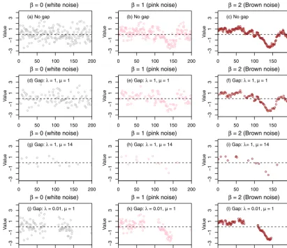
Figure 1.Synthetic time series with 200 time steps for three representative fractal scaling processes that correspond to white noise (β=0), pink noise (β=1), and Brown noise (β= 2).(a–c)show the simulated time series without any gap.(d–l)show the same time series as in(a–c)but with data gaps that were simulated using three different negative binomial (NB) distributions – that is,(d–f): NB(λ=1,µ=1);
(g–i): NB(λ=1,µ=14);(j–l): NB(λ=0.01,µ=1).
one, and two, the underlying processes are termed as “white”, “pink” (or “flicker”), and “Brown” (or “red”) noises, respec-tively (Witt and Malamud, 2013). Illustrative examples of these three noises are shown in Fig. 1a–c.
In addition, it can be shown that the spectral density func-tion for ARFIMA (p,d,q) is
f (ω)= σ
2
ε
2π
ψ (e−iω)
2
ϕ(e−iω)
2
1−e
−iω
−2d
(9)
for−π < ω < π (Boutahar et al., 2007; Beran et al., 2013).
For|ω| 1, Eq. (9) can be approximated by
f (ω)=C4|ω|−2d (10)
with
C4=
σε2
2π
|ψ (1)|2
|ϕ(1)|2. (11)
Equation (10) thus exhibits the asymptotic behavior required for a long-memory process given by Eq. (3). In addition, a comparison of Eqs. (10) and (8) reveals that
β=2d. (12)
Overall, these derivations indicate that these different types of scaling parameters (i.e., α, d, and H and β) can be used equivalently to describe the strength of fractal scaling. Specifically, their equivalency can be summarized as follows:
β=2d=1−α=2H−1. (13)
It should be noted, however, that the parametersd,α, and H are only applicable over a fixed range of fractal scaling, which is equivalent to (−1, 1) in terms ofβ.
1.3 Motivation and objective of this work
time series. Numerous estimation methods have been devel-oped for this purpose, including the Hurst rescaled range analysis, Higuchi’s method, Geweke and Porter-Hudak’s method, Whittle’s maximum likelihood estimator, detrended fluctuation analysis, and others (Taqqu et al., 1995; Monta-nari et al., 1997, 1999; Rea et al., 2009; Stroe-Kunold et al., 2009). For brevity, these methods are not elaborated here; readers are referred to Beran (2010) and Witt and Malamud (2013) for details. While these estimation methods have been extensively adopted, they are unfortunately only applicable to regular (i.e., evenly spaced) data, e.g., daily streamflow discharge, monthly temperature. In practice, many types of hydrological data, including river water-quality data, are of-ten sampled irregularly or have missing values, and hence their strengths of fractal scaling cannot be readily estimated with the above traditional estimation methods.
Thus, estimation of fractal scaling in irregularly sampled data is an important challenge for hydrologists and practi-tioners. Many data analysts may be tempted to interpolate the time series to make it regular and hence analyzable (Graham, 2009). Although technically convenient, interpolation can be problematic if it distorts the series’ autocorrelation structure (Kirchner and Weil, 1998). In this regard, it is important to evaluate various types of interpolation methods using care-fully designed benchmark tests and to identify the scenarios under which the interpolated data can yield reliable (or, al-ternatively, biased) estimates of spectral slope.
Moreover, quantification of fractal scaling in real-world water-quality data is subject to several common complexi-ties. First, water-quality data are rarely normally distributed; instead, they are typically characterized by log-normal or other skewed distributions (Hirsch et al., 1991; Helsel and Hirsch, 2002), with potential consequences forβestimation. Moreover, water-quality data also tend to exhibit long-term trends, seasonality, and flow dependence (Hirsch et al., 1991; Helsel and Hirsch, 2002), which can also affect the accuracy of β estimates. Thus, it may be more plausible to quantify β in transformed time series after accounting for the sea-sonal patterns and discharge-driven variations in the origi-nal time series, which is the approach taken in this paper. For the trend aspect, however, it remains a puzzle whether the data set should be detrended before conducting β esti-mation. Such detrending treatment can certainly affect the estimated value ofβand hence the validity of (or confidence in) any inference made regarding the statistical significance of temporal trends in the time series. This somewhat circu-lar issue is beyond the scope of our current work – it has been previously discussed in the context of short-term mem-ory (Zetterqvist, 1991; Darken et al., 2002; Yue et al., 2002; Noguchi et al., 2011; Clarke, 2013; Sang et al., 2014), but it is not well understood in the context of fractal scaling (or long-term memory) and hence presents an important area for future research.
In the above context, the main objective of this work was to use Monte Carlo simulation to systematically evaluate and
compare two broad types of approaches for estimating the strength of fractal scaling (i.e., spectral slopeβ) in irregularly sampled river water-quality time series. Specific aims of this work include the following:
1. to examine the sampling irregularity of typical river water-quality monitoring data and to simulate time se-ries that contain such irregularity, and
2. to evaluate two broad types of approaches for estimating βin simulated irregularly sampled time series.
The first type of approach includes several forms of interpo-lation techniques for gap filling, thus making the data reg-ular and analyzable by traditional estimation methods. The second type of approach includes the well-known Lomb– Scargle periodogram (Lomb, 1976; Scargle, 1982) and a recently developed wavelet method combined with a spec-tral aliasing filter (Kirchner and Neal, 2013). The latter two methods can be directly applied to irregularly spaced data; here we aim to compare them with the interpolation tech-niques. Details of these various approaches are provided in Sect. 3.1.
This work was designed to make several specific contri-butions. First, it uses benchmark tests to quantify the perfor-mance of a wide range of methods for estimating fractal scal-ing in irregularly sampled water-quality data. Second, it pro-poses an innovative and general approach for modeling sam-pling irregularity in water-quality records. Third, while this work was not intended to compare all published estimation methods for fractal scaling, it does provide and demonstrate a generalizable framework for data simulation (with gaps) and β estimation, which can be readily applied toward the eval-uation of other methods that are not covered here. Last but not least, while this work was intended to help hydrologists and practitioners understand the performance of various proaches for water-quality time series, the findings and ap-proaches may be broadly applicable to irregularly sampled data in other scientific disciplines.
The rest of the paper is organized as follows. We propose a general approach for modeling sampling irregularity in typ-ical river water-quality data and discuss our approach for simulating irregularly sampled data (Sect. 2). We then intro-duce various methods for estimating fractal scaling in irreg-ular time series and compare their estimation performance (Sect. 3). We close with a discussion of the results and impli-cations (Sect. 4).
2 Quantification of sampling irregularity in river water-quality data
2.1 Modeling of sampling irregularity
pe-riods; here we will address the implications of the irregular-ity, but not the (intentional) bias, inherent in such a sampling strategy. In other cases, the sampling is planned with a fixed sampling interval (e.g., 1 day) but samples are missed (or lost, or fail quality-control checks) at some time steps during implementation. In still other cases, the sampling is intrinsi-cally irregular because, for example, one cannot measure the chemistry of rainfall on rainless days or the chemistry of a stream that has dried up. Theoretically, any deviation from fixed-interval sampling can affect the subsequent analysis of the time series.
To quantify sampling irregularity, we propose a simple and general approach that can be applied to any time series of monitoring data. Specifically, for a given time series withN points, the time intervals between adjacent samples are cal-culated; these intervals themselves make up a time series of N-1 points that we call1t. For this time series, the following parameters are calculated to quantify its sampling irregular-ity:
– L=the length of the period of record; – N=the number of samples in the record;
– 1tnominal=the nominal sampling interval under regular sampling (e.g.,1tnominal=1 day for daily samples);
– 1t∗=1t / 1t
nominal, the sample intervals non-dimensionalized by the nominal sampling interval; – 1taverage=L /(N – 1) the average of all the entries in
1t.
The quantification is illustrated with two simple examples. The first example contains data sampled every hour from 01:00 to 11:00 UTC on 1 day. In this case,L=10 h,N=11 samples,1t={1, 1, 1, 1, 1, 1, 1, 1, 1, 1} h, and1tnominal= 1taverage=1 h. The second example contains data sampled at 01:00, 03:00, 04:00, 08:00, and 11:00. In this case,L=10 h, N=5 samples, 1t={2, 1, 4, 3} h, 1tnominal=1 h, and 1taverage=2.5 h. It is readily evident that the first case corre-sponds to fixed-interval (regular) sampling that has the prop-erty of1taverage/ 1tnominal=1 (dimensionless), whereas the second case corresponds to irregular sampling for which 1taverage/ 1tnominal> 1.
The dimensionless set1t∗contains essential information for determining sampling irregularity. This set is modeled as independent, identically distributed values drawn from a neg-ative binomial (NB) distribution. This distribution has two dimensionless parameters, the shape parameter (λ) and the mean parameter (µ), which collectively represent the irregu-larity of the samples. The NB distribution is a flexible distri-bution that provides a discrete analogue of a gamma distribu-tion. The geometric distribution, itself the discrete analogue of the exponential distribution, is a special case of the NB distribution whenλ=1.
The parameters µ and λ represent different aspects of sampling irregularity, as illustrated by the examples shown in Fig. 2. The mean parameter µ represents the fractional increase in the average interval between samples due to gaps: µ=mean(1t∗)−1 =(1taverage− 1tnominal) / 1tnominal. Thus, the special case of µ=0 cor-responds to regular sampling (i.e., 1taverage=1tnominal), whereas any larger value ofµcorresponds to irregular sam-pling (i.e.,1taverage>1tnominal) (Fig. 2c). The shape param-eterλcharacterizes the similarity of gaps to each other; that is, a smallλindicates that the samples contain gaps of widely varying lengths, whereas a largeλindicates that the samples contain many gaps of similar lengths (Fig. 2a, b).
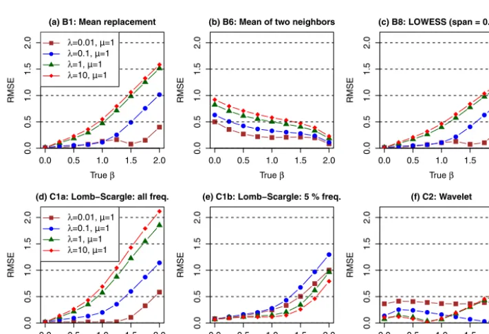
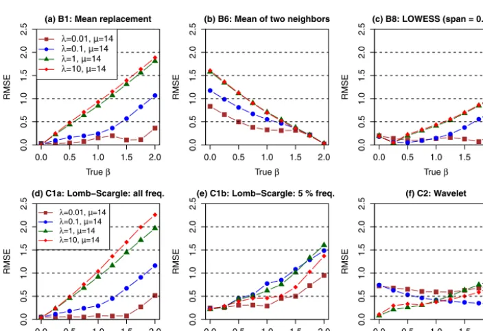
To visually illustrate these gap distributions, representative samples of irregular time series are presented in Fig. 1 for the three special processes described above (Sect. 1.2), i.e., white noise, pink noise, and Brown noise. Specifically, three differ-ent gap distributions, namely, NB(λ=1,µ=1), NB(λ=1, µ=14), and NB(λ=0.01,µ=1), were simulated and each was applied to convert the three original (regular) time se-ries (Fig. 1a–c) to irregular time sese-ries (Fig. 1d–1l). These simulations clearly illustrate the effects of the two parame-tersλandµ. In particular, compared with NB(λ=1,µ=1), NB(λ=1,µ=14) shows a similar level of sampling irregu-larity (sameλ) but a much longer average gap interval (larger µ). Again compared with NB(λ=1, µ=1), NB(λ=0.01, µ=1) shows the same average interval (sameµ) but a much more irregular (skewed) gap distribution that contains a few very large gaps (smallerλ).
2.2 Examination of sampling irregularity in real river water-quality data
T
able
1.
Quantification
of
sampling
irre
gularity
for
selected
w
ater
-quality
constituents
at
nine
sites
of
the
Chesapeak
e
Bay
Ri
v
er
Input
Monitoring
Program
and
six
sites
of
the
Lak
e
Erie
and
Ohio
T
rib
utary
Monitoring
Program.
(
λ
:
shape
parameter
estimated
using
maximum
lik
elihood;
λ
0
:
shape
parameter
esti
mated
using
the
direct
approach
(see
Sect.
2.2);
µ
:
mean
parameter;
1t
av
erage
:
av
erage
g
ap
interv
al;
N
:
total
number
of
samples.)
I.
Chesapeak
e
Bay
Ri
v
er
Input
Monitoring
program
Site
ID
Ri
v
er
and
station
name
Drainage
area
(km
2
)
T
otal
nitrogen
(TN)
T
otal
phosphorus
(TP)
λ
λ
0
µ
1t
av
erage
(days)
N
λ
λ
0
µ
1t
av
erage
(days)
N
01578310
Susquehanna
Ri
v
er
at
Cono
wingo,
MD
70
189
0.8
1.1
13.5
14.5
876
0.8
1.0
13.4
14.4
881
01646580
Potomac
Ri
v
er
at
Chain
Bridge,
W
ashington
D.C.
30
044
0.9
0.6
9.5
10.5
1385
1.1
1.0
24.4
25.4
579
02035000
James
Ri
v
er
at
Cartersville,
V
A
16
213
0.8
1.0
13.9
14.9
960
0.8
1.1
13.7
14.7
974
01668000
Rappahannock
Ri
v
er
near
Fredericksb
ur
g,
V
A
4144
0.8
0.6
15.6
16.6
776
0.8
0.6
15.2
16.2
796
02041650
Appomattox
Ri
v
er
at
Matoaca,
V
A
3471
0.8
0.8
15.1
16.1
798
0.8
0.8
14.9
15.9
810
01673000
P
amunk
ey
Ri
v
er
near
Hano
v
er
,
V
A
2774
0.8
0.9
15.1
16.1
873
0.8
1.0
14.7
15.7
894
01674500
Mattaponi
Ri
v
er
near
Beulahville,
V
A
1557
0.7
0.9
14.3
15.3
810
0.8
0.9
14.2
15.2
820
01594440
P
atux
ent
Ri
v
er
at
Bo
wie,
MD
901
0.9
1.1
15.3
16.3
787
0.8
0.8
14.0
15.0
861
01491000
Choptank
Ri
v
er
near
Greensboro,
MD
293
1.2
1.5
19.6
20.6
680
1.1
1.0
20.5
21.5
690
II.
Lak
e
Erie
and
Ohio
trib
utary
monitoring
program
Site
ID
Ri
v
er
and
station
name
Drainage
area
(km
2
)
Nitrate-plus-nitrite
(NO
x
)
T
otal
phosphorus
(TP)
λ
λ
0
µ
1t
av
erage
(days)
N
λ
λ
0
µ
1t
av
erage
(days)
N
04193500
Maumee
Ri
v
er
at
W
aterville,
OH
16
395
0.005
0.0003
0.19
1.19
9101
0.005
0.0003
0.19
1.19
9101
04198000
Sandusk
y
Ri
v
er
near
Fremont,
OH
3245
0.01
0.003
0.22
1.22
9641
0.01
0.003
0.22
1.22
9655
04208000
Cuyahog
a
Ri
v
er
at
Independence,
OH
1834
0.007
0.006
0.13
1.13
7421
0.007
0.006
0.13
1.13
7426
04212100
Grand
Ri
v
er
near
P
ainesville,
OH
1777
0.01
0.005
0.21
1.21
5023
0.01
0.005
0.22
1.22
4994
04197100
Hone
y
Creek
at
Melmore,
OH
386
0.007
0.005
0.06
1.06
9914
0.007
0.005
0.06
1.06
9914
04197170
Rock
Creek
at
T
if
fin,
OH
90
0.007
0.008
0.06
1.06
8422
0.007
0.008
0.06
1.06