Scale effect on overland flow connectivity at the plot scale

(1)

Hydrol. Earth Syst. Sci., 17, 87–101, 2013 www.hydrol-earth-syst-sci.net/17/87/2013/ doi:10.5194/hess-17-87-2013

Hydrology and

Earth System

Sciences

Scale effect on overland flow connectivity at the plot scale

A. Pe ˜nuela1, M. Javaux1,2, and C. L. Bielders1

1_{Earth and Life Institute, Universit´e catholique de Louvain, Croix du Sud 2, L7.05.02, 1348 Louvain-la-Neuve, Belgium} 2_{Agrosphere, IBG-3, Forschungszentrum Julich GmbH, 52425 Julich, Germany}

Correspondence to: A. Pe˜nuela ([email protected])

Received: 5 June 2012 – Published in Hydrol. Earth Syst. Sci. Discuss.: 25 June 2012 Revised: 30 November 2012 – Accepted: 7 December 2012 – Published: 14 January 2013

Abstract. A major challenge in present-day hydrological sci-ences is to enhance the performance of existing distributed hydrological models through a better description of sub-grid processes, in particular the subsub-grid connectivity of flow paths. The Relative Surface Connection (RSC) function was proposed by Antoine et al. (2009) as a functional indicator of runoff flow connectivity. For a given area, it expresses the percentage of the surface connected to the outflow boundary (C) as a function of the degree of filling of the depression storage. This function explicitly integrates the flow network at the soil surface and hence provides essential information regarding the flow paths’ connectivity. It has been shown that this function could help improve the modeling of the hydro-graph at the square meter scale, yet it is unknown how the scale affects the RSC function, and whether and how it can be extrapolated to other scales. The main objective of this research is to study the scale effect on overland flow connec-tivity (RSC function). For this purpose, digital elevation data of a real field (9×3 m) and three synthetic fields (6×6 m) with contrasting hydrological responses were used, and the RSC function was calculated at different scales by changing the length (l) or width (w) of the field. To different extents depending on the microtopography, border effects were ob-served for the smaller scales when decreasinglorw, which resulted in a strong decrease or increase of the maximum de-pression storage, respectively. There was no scale effect on the RSC function when changingw, but a remarkable scale effect was observed in the RSC function when changingl. In general, for a given degree of filling of the depression storage,C decreased asl increased, the change in C being inversely proportional to the change inl. However, this ob-servation applied only up to approx. 50–70 % (depending on the hydrological response of the field) of filling of depression storage, after which no correlation was found betweenCand

l. The results of this study help identify the minimal scale to study overland flow connectivity. At scales larger than the minimal scale, the RSC function showed a great potential to be extrapolated to other scales.

1 Introduction

The concept of connectivity, applied in many disciplines, aims at characterizing the behavior of heterogeneous systems according to the intrinsic organization of the heterogeneities. In the context of landscape connectivity, connectivity can be defined as the degree to which the landscape facilitates or impedes movement between resource patches (Taylor et al., 1993). In hydrology there is still no consensus about the definition of hydrological connectivity (Bracken and Croke, 2007; Ali and Roy, 2009). However, by analogy with the con-cept of landscape connectivity, overland flow connectivity can be defined as the degree to which the surface morphology facilitates or impedes overland flow. This definition, as well as the landscape connectivity concept, integrates two sub-concepts: structural and functional connectivity (Tischendorf and Fahring, 2000). Structural connectivity describes the ex-tent to which the surface morphology units, such as depres-sions, are linked to each other. It can be derived from topo-graphical information. Functional connectivity describes the effect produced by the surface morphology on the process of overland flow. Functional connectivity must therefore be de-rived from a combination of topographical information and hydrological modeling.

(2)

88 A. Pe ˜nuela et al.: Scale effect on overland flow connectivity at the plot scale

of the area of study. At the finest scale, soil roughness plays an important role through its effect on flow velocity. This ex-tensively studied effect is incorporated in hydrological mod-els as a friction factor. As the scale increases, the surface morphology increasingly influences overland flow (Darboux et al., 2002b). Indeed, the surface microtopography exerts a control over the infiltration process through its effects on the spatial heterogeneity of surface sealing (Langhans et al., 2011). Furthermore, the spatial configuration of the system, formed by water-contributing sources, water-accepting sinks (depressions) and connecting links (e.g., small rills between depressions), determines the hydrological response of the system. The study of the spatial configuration by geostatistics (e.g., the semivariogram) or landscape metrics allows com-parison and classification of dominant processes and may partly explain the hydrological response. However, it is not adequate for predictive purposes in terms of hydrological re-sponse and connectivity (Van Nieuwenhuyse et al., 2011).

From the hillslope to the small watershed scale, distributed hydrological models frequently use “plot size” (1–1000 m2) grid cells allowing for an explicit analysis of overland flow connectivity. However, such hydrological models do not ex-plicitly treat overland flow connectivity below the grid cell size. Overland flow processes in each grid cell are generally represented by two effective parameters, the maximum de-pression storage (i.e., maximum volume of water that the soil is able to store in surface depressions) and the friction factor (i.e., resistance to flow) (Singh and Frevert, 2002; Smith et al., 2007), which have been found neither to reflect overland flow processes realistically at the subgrid scale nor to allow for proper discrimination between different hydrological re-sponses (Antoine et al., 2009).

Generally, hydrological models assume that the generation of overland flow only starts after the maximum depression storage is reached (Singh and Frevert, 2002). However, this assumption underestimates the surface connected to down-stream areas and hence the volume of runoff generated before the complete filling of depressions (Antoine et al., 2011). In reality, depressions progressively overflow and water flows either to nearby depressions, or to the outflow boundary (On-stad, 1984; Darboux et al., 2002b). As depression storage in-creases, a larger area of the field becomes connected and con-tributes to the overland flow generation. This gradual process delays the initiation of the overland flow, and hence of the hy-drograph. A better understanding of the connectivity dynam-ics, which drive the hydrological response of a system at dif-ferent scales (Lexartza-Artza and Wainwright, 2009), should improve current hydrological modeling and runoff prediction (Western et al., 2001; Mueller et al., 2007).

In order to fully take into account overland flow connec-tivity at the hillslope and small watershed scale, it would be necessary to provide hydrological models with subgrid mi-crotopographical information. The use of a high resolution DEM (cm–mm resolution) in hydrological models would strongly increase the input data and the computation time

requirements. Yet even more problematic would be the acqui-sition of such data over large areas. Hence, subgrid connec-tivity functions, able to differentiate between different sur-face morphologies having different hydrological responses, must be developed in order to improve the prediction of flows at the hillslope and small watershed-scale scale without crit-ically increasing computation time and data requirements of distributed hydrological models.

As subgrid connectivity is expected to be scale-dependent, extra attention must be paid in order to select an appropriate size of the grid cell. Some studies have reported the existence of a representative elementary area (Wood et al., 1988) or length scale (Julien and Moglen, 1990) that could serve to de-termine the grid cell scale in hydrological models. Firstly, the grid cell must be sufficiently large to be representative of the process of overland flow connectivity at the plot scale, i.e., all the components and the relationships between them must be represented (Ali and Roy, 2009). Secondly, it must minimize border effects so as to neither miss nor modify some of these components. In addition, slope length has been observed to influence the response of the overland flow, showing a lower runoff coefficient with increasing length (Van de Giessen et al., 2000; Cerdan et al., 2004). It has generally been assumed that this results from the spatial variability of rainfall and in-filtration capacity (Yair and Lavee, 1985). Yet this effect has also been observed on homogenous hillslopes, in which case it was attributed to a change in residence time (Stomph et al., 2002). According to the definition of overland flow connec-tivity mentioned above, connecconnec-tivity is expected to decrease with increasing slope lengths, since the probability for the water flow to encounter depressions is higher. However, the effect of slope length on overland flow connectivity and the runoff coefficient is still unclear.

In order to analyze and quantify the effect of scale on over-land flow connectivity, a functional connectivity indicator was selected, the so-called Relative Surface Connection (RSC) function (Antoine et al., 2009). It expresses the per-centage of the surface connected to the outflow boundary of a grid element as a function of the degree of filling of the depression storage. This function explicitly integrates the flow network at the soil surface and hence provides essen-tial information regarding the flow paths’ connectivity. It can be calculated much faster than the full resolution of the St. Venant equations and it has shown good results in captur-ing runoff-relevant connectivity properties compared to other connectivity indicators (Antoine et al., 2009). By adding sur-face detention dynamics to the RSC function (Antoine et al., 2011), this connectivity function also allowed to simulate in a simple way experimental hydrographs. Moreover, it could potentially be integrated in hydrological models in a man-ner similar to the Probability Density Model (PDM) (Moore, 2007), which implements the subgrid variability of the “soil absorption capacity” as a probability density curve.

The RSC function showed very promising results at the square meter scale but, as a functional connectivity indicator,

(3)

A. Pe ˜nuela et al.: Scale effect on overland flow connectivity at the plot scale 89

it may be scale-dependent and affected by border effects. However, it is unknown how changes in scale affect the RSC function and whether and how the RSC function can be ex-trapolated to other scales.

The objective of this study is therefore twofold. The first objective is to study the effect of changing scale on the RSC function for scales ranging from 0.18 m2to 36 m2. The sec-ond objective is to investigate the potential of the RSC func-tion to be extrapolated to larger scales. For these purposes, the RSC function will be calculated and compared at dif-ferent scales and for difdif-ferent microtopography types. The present study focuses on the hydrological connectivity at the plot scale, considering no interferences from infiltration, i.e., the infiltration capacity of the soil is assumed to be spatially homogeneous, constant over time and lower than the rainfall intensity. These assumptions, which do not take into account the effect of the spatial heterogeneity of the soil hydraulic conductivity on surface runoff (Langhans et al., 2011), nev-ertheless facilitate the study of the effects of the surface mor-phology and scale on overland flow.

2 Materials and method

2.1 Characteristics of the microtopographies

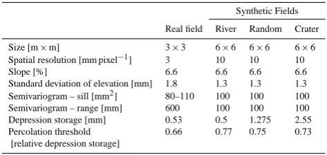
Two types of DEMs were used, real and synthetic. First, we used the DEM from a field located near Fort Collins, Colorado (USA), obtained by laser scanning (courtesy of the USDA-ARS Agricultural Systems Research Unit in Fort Collins). The field had been under grassland but the grass had been killed chemically and left to decay before scanning. The total size of the DEM is 9.5 m×4.8 m, the spatialx-y reso-lution is 1.5 mm and the vertical resoreso-lution is 0.5 mm. The natural slope of the field is 6.6 %. In order to avoid border effects that may have been generated during the process of obtaining the DEM, this study focuses on the central area, with a size of 9 m×3 m. This was also guided by the need to have three square replicate areas of the largest possible size (in this case, 3 m×3 m). For computational reasons, the spa-tialx-y resolution of the DEM was reduced to 3 mm. The semi-variograms of the three replicates had a range of ap-proximately 600 mm and a sill of 80–110 mm2(Table 1).

[image:3.595.310.547.81.193.2]

Secondly, in order to evaluate the scale effect in scenar-ios with different hydrological characteristics and connectiv-ity patterns, synthetic fields with contrasting microtopogra-phies were generated using a method developed by Zinn and Harvey (2003) and adapted by Antoine et al. (2009). The synthetic fields present identical statistics in terms of mean elevation, standard deviation and semivariogram. How-ever, they have different connectivity patterns. This method also allowed us to study the scale effect at larger scales compared to the real field case, yet the size of the fields was nevertheless limited for computational reasons. Three different types of microtopographies were generated using

Table 1. Main characteristics of the microtopographies.

Synthetic Fields Real field River Random Crater

Size [m×m] 3×3 6×6 6×6 6×6

Spatial resolution [mm pixel−1] 3 10 10 10

Slope [%] 6.6 6.6 6.6 6.6

Standard deviation of elevation [mm] 1.8 1.3 1.3 1.3 Semivariogram – sill [mm2] 80–110 100 100 100

Semivariogram – range [mm] 600 100 100 100

Depression storage [mm] 0.53 0.5 1.275 2.55

Percolation threshold 0.66 0.77 0.75 0.73

[relative depression storage]

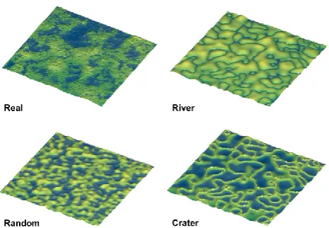
this method: (a) “river”, (b) “crater” and (c) “random” type (Fig. 1; Antoine et al., 2009). The “river” type microtopog-raphy presents high areas connected by a system of rills. On the other hand, the “crater” type, which is the reverse of the river type, presents a system of crests that isolate the depressions from each other. The “random” type mi-crotopography is an intermediate scenario represented by a standard multi-Gaussian synthetic field. The three synthetic fields are characterized by values of sill (100 mm2) and range (100 mm) of the semivariogram also observed in real fields (Vidal Vazquez et al., 2005) and experimental plots (Darboux et al., 2002b). A slope equal to the natural slope (6.6 %) of the real field was also added.

2.2 Filling algorithm and Relative Surface Connection (RSC) function

A filling algorithm (Antoine et al., 2009) was used to evaluate the overland flow connectivity. This method calculates a sim-plified hydrograph in which the velocity of the water is infi-nite and infiltration is not considered. A uniform rainfall is applied over the digital elevation model (DEM) of the study area. At every time step, a certain volume of water is applied in every pixel of the DEM. These volumes of water “walk” over the DEM to the lowest pixel selected by an 8-neighbor scheme until they reach a depression or the outflow bound-ary. In a depression, this volume of water is stored as depres-sion storage. Once the depresdepres-sion overflows, any excess of water flows to the next depression or to the outflow bound-ary. Since the water velocity is infinite, surface detention, i.e. water that is not trapped in depressions, is removed at every time step (Antoine et al., 2012). When a drop reaches the out-flow boundary it is added to the hydrograph. Since both the infiltration and the transfer time are nil, the ratio of instanta-neous outflow to the instantainstanta-neous inflow corresponds to the percentage of the total area connected to the outflow bound-ary (C). Thus, this ratio will be equal to 1 when 100 % of the surface of the study area is connected to the outflow bound-ary. At that point, depression storage reaches its maximum value, i.e., the dead storage zone is completely filled.

(4)

Fig. 1. Detail of the four microtopography types (2 m×2 m) with depressions partially filled with water (in blue) in order to highlight the contrasting connectivities.

the cumulative input of water. In this case, the area under the simplified hydrograph is equal to the cumulative volume of outflow [m3] and the area betweenC= 1 and the simplified hydrograph corresponds to the MDS (maximum depression storage). Based on this, we can representC as a function of the depression storage (Fig. 2). This is known as the Relative Surface Connection (RSC) function, which is a functional connectivity indicator that is able to discriminate well among surfaces with differing levels of connectivity and that can po-tentially be implemented in hydrological models (Antoine et al., 2009).

2.3 Process of plot fragmentation and calculation of the RSC function

Two different scale effects were considered, i.e., changing the width of the plot area and changing the length of the plot area. Therefore, the area was first divided into narrower ar-eas (from 1/2 up to 1/32 of the initial width) keeping the ini-tial length constant, and secondly the area was divided into shorter areas (from 1/2 up to 1/32 of the initial length) keep-ing the initial width constant (Fig. 3). The process of frag-mentation of the plots and the calculation of the RSC func-tion was exactly the same for all the fields. After the plot areas were divided, the filling algorithm was run in each of these sub-areas in order to obtain their RSC function. Finally, for a given scale, the RSC functions obtained in each sub-area were averaged in order to compare overland flow con-nectivity at different scales.

2.4 Representative width and length

In order to identify the minimal scale at which overland flow connectivity can be studied, a representative width and length were defined. Since border effects are expected to mainly cause variations in the MDS of the field, the representative

25 1

Figure 2: Example of Relative Surface Connection (RSC) function and connectivity evolution 2

(areas connected to the bottom boundary are shown in black). 3

4

5

6

7

8

9

10

11

12

0 1 2 3

0 0.2 0.4 0.6 0.8 1

Depression storage [mm]

C

[

m

3s -1/m 3s -1]

=

ra

ti

o

f

s

u

rf

.

c

o

n

e

c

te

d

[

m

2/m 2]

Fig. 2. Example of Relative Surface Connection (RSC) function and connectivity evolution (areas connected to the bottom boundary are shown in black).

width and length will be defined in function of the observed change in the MDS. Although the full width and legth of the plot are needed to estimate the MDS with the highest accu-racy, in practice, a small error on the estimation of the MDS may be acceptable. This acceptable error was arbitrarily set at 10 % of the MDS whenw→ ∞orl→ ∞in the present study. The value of the corresponding width and length will be referred to as the “representative width” (Table 2) and “representative length” (Table 3), and will be used to quantify and compare the scale effects between the four microtopog-raphy types.

3 Results 3.1 Real field

3.1.1 Scale effect produced by changing only the width When representing the average RSC function for each width in the same graph (Fig. 4a), a gradual shift of the RSC func-tion to the left is observed, indicating a gradual decrease of the MDS with increasing width. This decrease in MDS is in-versely proportional to the width, tending asymptotically to a constant value (Fig. 4b). This can be represented adequately by the following expression (Eq. 1):

MDS(w)= k

w+v, (1)

where MDS is the maximum depression storage [mm] for a given width w [mm] of the plot, k [mm] is a constant (Table 2) whose value reflects the magnitude of the asymp-totic decrease of the MDS when increasing the width of the plot, and v represents the MDS when w tends to infinity (MDSw→∞).

[image:4.595.311.544.64.223.2] [image:4.595.53.286.66.227.2]

(5)

[image:5.595.314.539.60.403.2]

26 1

Figure 3: Division pattern when changing (a) width and (b) length of the plots. 2

3

4

5

6

7

8

9

10

11

12

Fig. 3. Division pattern when changing (a) width and (b) length of the plots.

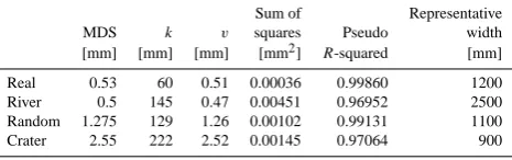
Table 2. Parameters of Eq. (1) when changing width (w), good-ness of fit expressed as the sum of squares (SS) and the pseudo

R-squared, and representative width for the four microtopography

types.

Sum of Representative

MDS k v squares Pseudo width

[mm] [mm] [mm] [mm2_] _R-squared _[mm]

Real 0.53 60 0.51 0.00036 0.99860 1200

River 0.5 145 0.47 0.00451 0.96952 2500

Random 1.275 129 1.26 0.00102 0.99131 1100

Crater 2.55 222 2.52 0.00145 0.97064 900

A “representative width” can be defined based on an ac-ceptable error of 10 % on MDSw→∞(Table 3). This

accept-able error is represented in Fig. 4b as dashed lines.

In order to compare the shape of the different RSC func-tions, the depression storage was normalized by the value of the maximum depression storage for each scale (Fig. 5). This way of representing the RSC function shows that the shape is little affected by width except for the two smallest scales (width = 0.188 m and 0.09 m), which present a strong deviation in the last third of the function (relative depres-sion storage approximately>2/3). These two curves show a displacement to the right, i.e., for the same value of rela-tive depression storage the connectivity is lower for the two smallest scales as compared to the larger scales.

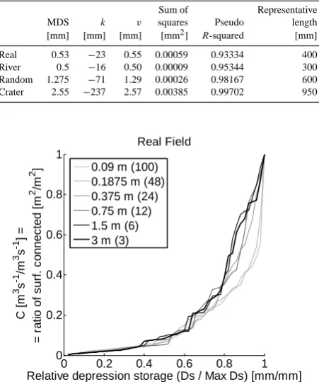
3.1.2 Scale effect produced by changing only the length When changing the length for a constant width of 3 m, the average RSC functions show the opposite trend than was ob-served when changing the width. The RSC function shows a gradual shift to the right as the plot length increases (Fig. 6a), i.e., a gradual increase of the MDS with increasing length. This increase in MDS with plot length can also be fitted ad-equately by Eq. (1), after replacing w byl and with k <0 (Fig. 6b). The corresponding parameters are provided in Ta-ble 3. In this case,v represents the MDS when l tends to infinity (MDSl→∞).

27

1

2

Figure 4: Real field – Effect of plot width on the average RSC function (a) and on the 3

maximum depression storage (MDS) (b). The numbers in parentheses indicate the number of 4

connectivity curves used for calculating the average RSC functions. Vertical bars = standard 5

deviations. The arrow indicates the ‘representative width’. All the plots are 3 m long. 6

7

8

9

0 0.5 1 1.5

0 0.2 0.4 0.6 0.8 1

Real Field

C

[

m

3s -1/m 3s -1]

=

r

a

ti

o

f

s

u

rf

.

c

o

n

e

c

te

d

[

m

2 /m 2 ] (a)

0.09 m (100) 0.1875 m (48) 0.375 m (24) 0.75 m (12) 1.5 m (6) 3 m (3)

0 500 1000 1500 2000 2500 3000 0

0.2 0.4 0.6 0.8 1 1.2 1.4 1.6

Real Field

Width [mm]

M

a

x

im

u

m

D

e

p

re

s

io

n

S

to

ra

g

e

[

m

]

(b) Abs MDS

Abs MDS +/- 10% Fitted Curve

→ → +/- 10%

Equation 1

27

1

2

Figure 4: Real field – Effect of plot width on the average RSC function (a) and on the 3

deviations. The arrow indicates the ‘representative width’. All the plots are 3 m long. 6

7

8

9

0 0.5 1 1.5

0 0.2 0.4 0.6 0.8 1

Real Field

C

[

m

3 s -1 /m 3 s -1 ]

=

r

a

ti

o

f

s

u

rf

.

c

o

n

e

c

te

d

[

m

2 /m 2 ] (a)

0.09 m (100) 0.1875 m (48) 0.375 m (24) 0.75 m (12) 1.5 m (6) 3 m (3)

0 500 1000 1500 2000 2500 3000

0 0.2 0.4 0.6 0.8 1 1.2 1.4 1.6

Real Field

Width [mm]

M

a

x

im

u

m

D

e

p

re

s

io

n

S

to

ra

g

e

[

m

]

(b) _{Abs MDS}

Abs MDS +/- 10% Fitted Curve

→ → +/- 10%

Equation 1

Fig. 4. Real field – effect of plot width on the average RSC function (a) and on the maximum depression storage (MDS) (b). The num-bers in parentheses indicate the number of connectivity curves used for calculating the average RSC functions. Vertical bars = standard deviations. The arrow indicates the representative width. All the plots are 3 m long.

As was done for width, a “representative length” can be defined based on an acceptable error of 10 % on MDSl→∞

(Table 3). This acceptable error is represented in Fig. 6b as dashed lines.

[image:5.595.49.283.66.184.2] [image:5.595.52.285.294.367.2]

(6)

[image:6.595.315.539.65.424.2]

Table 3. Parameters of Eq. (1) when changing length (l), good-ness of fit expressed as the sum of squares (SS) and the pseudo

R-squared, and representative length for the four microtopography

types.

Sum of Representative

MDS k v squares Pseudo length

[mm] [mm] [mm] [mm2] R-squared [mm]

Real 0.53 −23 0.55 0.00059 0.93334 400

River 0.5 −16 0.50 0.00009 0.95344 300

Random 1.275 −71 1.29 0.00026 0.98167 600

Crater 2.55 −237 2.57 0.00385 0.99702 950

28 1

Figure 5: Real Field - Effect of plot width on the normalized RSC function. Depression 2

storage (x axis) was scaled by the maximum depression storage. The numbers in parentheses 3

indicate the number of connectivity curves used for calculating the average normalized RSC 4

functions. All the plots are 3 m long. 5

6

7

8

9

10

0 0.2 0.4 0.6 0.8 1

Real Field

Relative depression storage (Ds / Max Ds) [mm/mm]

C

[

m

3 s -1 /m 3 s -1 ]

=

r

a

ti

o

f

s

u

rf

.

c

o

n

e

c

te

d

[

m

2/m

2] 0.09 m (100)

0.1875 m (48) 0.375 m (24) 0.75 m (12) 1.5 m (6) 3 m (3)

Fig. 5. Real field – effect of plot width on the normalized RSC func-tion. Depression storage (x-axis) was scaled by the maximum de-pression storage. The numbers in parentheses indicate the number of connectivity curves used for calculating the average normalized RSC functions. All the plots are 3 m long.

3.2 Synthetic Fields

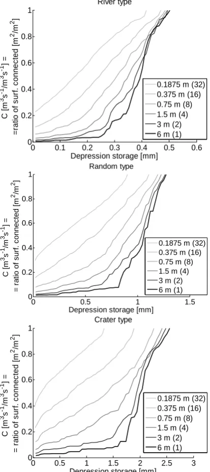
3.2.1 Scale effect produced by changing only the width As for the real field, when increasing the plot width, a grad-ual shift of the RSC function to the left is observed (Fig. 8), reflecting a gradual decrease of the MDS. MDS decreases asymptotically towards a constant value as the width is in-creased (Fig. 9), which can be represented adequately by Eq. (1). The corresponding parameters are provided in Ta-ble 2. MDSw→∞ increases gradually from the river to the

crater topography. As indicated by the k-values, the asymp-totic decrease of MDS with increasing widths is most pro-nounced for the crater microtopography. However, as the rep-resentative width is determined based on an acceptable rela-tive error of 10 % on the estimation of MDSw→∞, the river

microtopography is characterized by a higher representative width (2500 mm) as compared to the random and crater mi-crotopographies that show smaller yet similar representative widths (1100 mm and 900 mm respectively).

29

1

2

Figure 6: Real field – Effect of plot length on the average RSC function (a) and on the 3

deviations. The arrow indicates the ‘representative length’. All the plots are 3 m wide. 6

7

8

9

0 0.1 0.2 0.3 0.4 0.5 0.6

0 0.1 0.2 0.3 0.4 0.5 0.6 0.7 0.8 0.9 1

Real Field

C

[

m

3s -1/m 3s -1]

=

r

a

ti

o

f

s

u

rf

.

c

o

n

e

c

te

d

[

m

2/m 2]

(a)

0.09 m (100) 0.1875 m (48) 0.375 m (24) 0.75 m (12) 1.5 m (6) 3 m (3)

0 500 1000 1500 2000 2500 3000 0

0.1 0.2 0.3 0.4 0.5 0.6

Real Field

Length [mm]

M

a

x

im

u

m

D

e

p

re

s

io

n

S

to

ra

g

e

[

m

]

(b) Abs MDS Abs MDS +/- 10% Fitted Curve

→ → +/- 10% Equation 1

29

1

2

Figure 6: Real field – Effect of plot length on the average RSC function (a) and on the 3

deviations. The arrow indicates the ‘representative length’. All the plots are 3 m wide. 6

7

8

9

0 0.1 0.2 0.3 0.4 0.5 0.6

0 0.1 0.2 0.3 0.4 0.5 0.6 0.7 0.8 0.9 1

Real Field

C

[

m

3s -1/m 3s -1]

=

r

a

ti

o

f

s

u

rf

.

c

o

n

e

c

te

d

[

m

2/m 2]

(a)

0.09 m (100) 0.1875 m (48) 0.375 m (24) 0.75 m (12) 1.5 m (6) 3 m (3)

0 500 1000 1500 2000 2500 3000

0 0.1 0.2 0.3 0.4 0.5 0.6

Real Field

Length [mm]

M

a

x

im

u

m

D

e

p

re

s

io

n

S

to

ra

g

e

[

m

]

(b)

Abs MDS Abs MDS +/- 10% Fitted Curve

→ → +/- 10% Equation 1

Fig. 6. Real field – effect of plot length on the average RSC function (a) and on the maximum depression storage (MDS) (b). The num-bers in parentheses indicate the number of connectivity curves used for calculating the average RSC functions. Vertical bars = standard deviations. The arrow indicates the representative length. All the plots are 3 m wide.

The shape of the RSC function, as for the real field, is little affected by a change in width, except for the smallest values of width (Fig. 10). For the random and river types, this deviation is only observable at the two smallest scales (width = 0.375 m and 0.188 m) in the last third of the RSC function. For the crater type, a deviation is also noticeable in the last third of the RSC function for the intermediate widths (width = 0.75 m and 1.5 m).

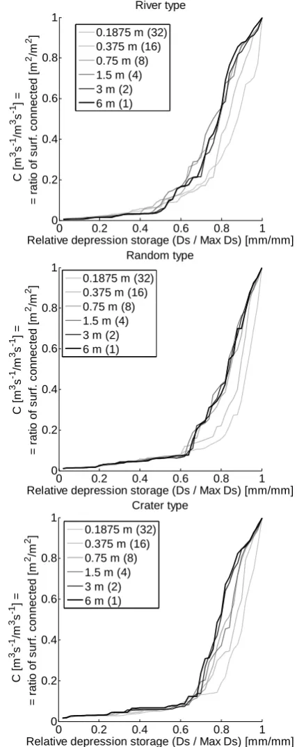
3.2.2 Scale effect produced by changing only the length When reducing the length and keeping the initial width (6 m), the average RSC functions show the opposite effect com-pared to when changing the width, just like the real field. Again, there is a gradual shift of the RSC to the right with in-creasing length (Fig. 11). The MDS increases asymptotically

[image:6.595.56.282.115.385.2]

(7)

30 1

Figure 7: Real Field - Effect of plot length on the normalized RSC function. Depression

2

storage (x axis) was scaled by the maximum depression storage. The numbers in parentheses

3

indicate the number of connectivity curves used for calculating the average normalized RSC

4

functions. All the plots are 3 m wide.

5 6 7 8 9 10 11 12 13 14 15 16

0 0.2 0.4 0.6 0.8 1

0 0.2 0.4 0.6 0.8 1 Real Field

Relative depression storage (Ds / Max Ds) [mm/mm]C

[ m 3 s -1 /m 3 s -1 ] = r a ti o o f s u rf . c o n n e c te d [ m 2 /m 2 ]

3 m x 0.09 m 3 m x 0.1875 m 3 m x 0.375 m 3 m x 0.75 m 3 m x 1.5 m 3 m x 3 m

Fig. 7. Real field – effect of plot length on the normalized RSC function. Depression storage (x-axis) was scaled by the maximum depression storage. The numbers in parentheses indicate the number of connectivity curves used for calculating the average normalized RSC functions. All the plots are 3 m wide.

towards a constant value as the length increases (Fig. 12), which can be fitted by Eq. (1) after replacingwbyl. The cor-responding values ofk(k <0) andvare given in Table 3. As indicated by the k-values, the river microtopography tends more rapidly to its asymptotic value than the random or crater microtopographies. The representative length increases from the river (300 mm) to the crater type (950 mm).

As for the real field, a reduction in length not only causes a decrease in MDS but also a change in the shape of the RSC functions. For a given value of the relative depres-sion storage, a decrease in connectivity is observed as the length increases (Fig. 13). The RSC function tends from a concave shape for the largest plot lengths to a straighter or even convex shape, especially for the smallest scales (length = 0.375 m and 0.188 m). The change in the shape of the RSC function is least pronounced for the river type and most pronounced for the crater type.

4 Discussion

4.1 Scale effect on the MDS

For all the cases studied, a gradual increase or decrease of the MDS has been observed when decreasing the width or the length, respectively. This can be explained by the increasing influence of the lateral and bottom boundaries when reduc-ing the scale, i.e., by two border effects. On the one hand, the reduction of the width causes the interruption of the con-necting paths between depressions (Figs. 4b and 9). Below a certain scale, the deviation of the MDS from the MDSw→∞

starts to be considerable. Below this scale, the area between the virtual lateral plot boundaries is not able to represent adequately all the components involved in the functional

31

1

2

3

Figure 8: Synthetic Fields – Effect of plot width on the averaged RSC function for the

4

“River”, “Random” and “Crater” type microtopographies. The numbers in parentheses

5

0 0.5 1 1.5

0 0.2 0.4 0.6 0.8 1 River type

C [ m 3s -1/m 3s -1] = = r a ti o o f s u rf . c o n n e c te d [ m 2 /m 2 ]

0.1875 m (32) 0.375 m (16) 0.75 m (8) 1.5 m (4) 3 m (2) 6 m (1)

0 0.5 1 1.5 2

0 0.2 0.4 0.6 0.8 1 Random type

C [ m 3 s -1 /m 3 s -1 ] = = r a ti o o f s u rf . c o n n e c te d [ m 2 /m

2 ] (a) 0.1875 m (32)

0.375 m (16) 0.75 m (8) 1.5 m (4) 3 m (2) 6 m (1)

0 1 2 3 4

0 0.2 0.4 0.6 0.8 1 Crater type

2 ] (a) 0.1875 m (32)

0.375 m (16) 0.75 m (8) 1.5 m (4) 3 m (2) 6 m (1)

31

1

2

3

4

5

0 0.5 1 1.5

0 0.2 0.4 0.6 0.8 1 River type

0.1875 m (32) 0.375 m (16) 0.75 m (8) 1.5 m (4) 3 m (2) 6 m (1)

0 0.5 1 1.5 2

0 0.2 0.4 0.6 0.8 1 Random type

C [ m 3s -1/m 3s -1] = = r a ti o o f s u rf . c o n n e c te d [ m 2 /m

2 ] (a) 0.1875 m (32)

0.375 m (16) 0.75 m (8) 1.5 m (4) 3 m (2) 6 m (1)

0 1 2 3 4

0 0.2 0.4 0.6 0.8 1 Crater type

2 ] (a) 0.1875 m (32)

0.375 m (16) 0.75 m (8) 1.5 m (4) 3 m (2) 6 m (1)

31

1

2

3

4

5

0 0.5 1 1.5

0 0.2 0.4 0.6 0.8 1 River type

C [ m 3s -1/m 3s -1] = = r a ti o o f s u rf . c o n n e c te d [ m 2/m 2]

0.1875 m (32) 0.375 m (16) 0.75 m (8) 1.5 m (4) 3 m (2) 6 m (1)

0 0.5 1 1.5 2

0 0.2 0.4 0.6 0.8 1 Random type

2 ] (a) 0.1875 m (32)

0.375 m (16) 0.75 m (8) 1.5 m (4) 3 m (2) 6 m (1)

0 1 2 3 4

0 0.2 0.4 0.6 0.8 1 Crater type

C [ m 3s -1/m 3s -1] = = r a ti o o f s u rf . c o n n e c te d [ m 2/m

2] (a) 0.1875 m (32)

0.375 m (16) 0.75 m (8) 1.5 m (4) 3 m (2) 6 m (1)

Fig. 8. Synthetic fields – effect of plot width on the averaged RSC function for the river, random and crater type microtopographies. The numbers in parentheses indicate the number of connectivity curves used for calculating the average RSC functions. All plots are 6 m long.

[image:7.595.66.275.65.229.2] [image:7.595.317.539.68.553.2]

(8)

[image:8.595.65.269.60.230.2] [image:8.595.319.533.64.602.2]

33 1

Figure 9: Synthetic Fields – Effect of plot width on the maximum depression storage for the 2

“River”, “Random” and “Crater” type microtopographies. Vertical bars = standard 3

deviations. The arrows indicate the ‘representative width’. All the plots are 6 m long. 4 5 6 7 8 9 10 11 12 13

0 2000 4000 6000

0 1 2 3 4 Crater Width [mm] M a x im u m D e p re s s io n S to ra g e [ m m ] (b) River Random Abs MDS Abs MDS +/- 10% Fitted Curve

→∞ →∞+/- 10% Equation 1

Fig. 9. Synthetic fields – effect of plot width on the maximum de-pression storage for the river, random and crater type microtopogra-phies. Vertical bars = standard deviations. The arrows indicate the representative width. All the plots are 6 m long.

the other hand, when the plot length is reduced below a cer-tain scale (Figs. 6b and 12), the resulting area becomes less and less representative of all the components that cause the accumulation of water in the depressions (i.e., barriers in the direction of flow). In other words, as the length decreases, a larger proportion of depressions gets crossed by the virtual downstream outflow boundary, and hence they get more eas-ily connected to it.

These two border effects affect all the microtopography types similarly in a qualitative way but differently in a quan-titative way. In order to quantify and compare these effects between the different microtopography types, a representa-tive scale was defined based on an acceptable deviation of the MDS by 10 % from its asymptotic value (Figs. 4b, 6b, 9, and 12). This representative scale represents the width or length below which the border effects start to be consider-able, i.e., the plot is neither long enough nor wide enough to be representative of the process of overland flow connectivity occurring at larger scales. A 10 % deviation from MDSw→∞

or MDSl→∞ was selected since smaller deviations of the

MDS would barely affect results in hydrological modeling. Indeed, in our study, MDSw→∞or MDSl→∞values ranged

from 0.5 mm to 2.5 mm, such that a 10 % relative error would lead to an absolute error comprised between 0.05 mm and 0.25 mm. We believe that having a greater accuracy on the MDS would not be relevant for most practical applications, whereas accepting a higher relative error, especially in fields with high values of MDS, might lead to a substantial bias in hydrograph estimation.

The proposed representative scale provides a measure of the sensitivity of the different microtopographies to these two border effects. It is calculated using Eq. (1) (Tables 2 and

3). When plotted as a function of MDSw→∞ or MDSl→∞ 34

1

2

3

Figure 10: Synthetic Fields – Effect of plot width on the average normalized RSC function for

4

the “River”, “Random” and “Crater” type microtopographies. Depression storage (x axis)

5

was scaled by the maximum depression storage. The numbers in parentheses indicate the

6

0 0.2 0.4 0.6 0.8 1

0 0.2 0.4 0.6 0.8 1 River type

C [ m 3s -1/m 3s -1] = = r a ti o o f s u rf . c o n n e c te d [ m 2/m

2] 0.1875 m (32)

0.375 m (16) 0.75 m (8) 1.5 m (4) 3 m (2) 6 m (1)

0 0.2 0.4 0.6 0.8 1

0 0.2 0.4 0.6 0.8 1 Random type

C [ m 3 s -1 /m 3 s -1 ] = = r a ti o o f s u rf . c o n n e c te d [ m 2 /m 2 ]

0.1875 m (32) 0.375 m (16) 0.75 m (8) 1.5 m (4) 3 m (2) 6 m (1)

0 0.2 0.4 0.6 0.8 1

0 0.2 0.4 0.6 0.8 1 Crater type

0.1875 m (32) 0.375 m (16) 0.75 m (8) 1.5 m (4) 3 m (2) 6 m (1)

34 1

2

3

Figure 10: Synthetic Fields – Effect of plot width on the average normalized RSC function for

4

the “River”, “Random” and “Crater” type microtopographies. Depression storage (x axis)

5

was scaled by the maximum depression storage. The numbers in parentheses indicate the

6

0 0.2 0.4 0.6 0.8 1

0 0.2 0.4 0.6 0.8 1 River type

2 ] 0.1875 m (32)

0.375 m (16) 0.75 m (8) 1.5 m (4) 3 m (2) 6 m (1)

0 0.2 0.4 0.6 0.8 1

0 0.2 0.4 0.6 0.8 1 Random type

0.1875 m (32) 0.375 m (16) 0.75 m (8) 1.5 m (4) 3 m (2) 6 m (1)

0 0.2 0.4 0.6 0.8 1

0 0.2 0.4 0.6 0.8 1 Crater type

0.1875 m (32) 0.375 m (16) 0.75 m (8) 1.5 m (4) 3 m (2) 6 m (1)

34 1

2

3

Figure 10: Synthetic Fields – Effect of plot width on the average normalized RSC function for

4

the “River”, “Random” and “Crater” type microtopographies. Depression storage (x axis)

5

was scaled by the maximum depression storage. The numbers in parentheses indicate the

6

0 0.2 0.4 0.6 0.8 1

0 0.2 0.4 0.6 0.8 1 River type

2 ] 0.1875 m (32)

0.375 m (16) 0.75 m (8) 1.5 m (4) 3 m (2) 6 m (1)

0 0.2 0.4 0.6 0.8 1

0 0.2 0.4 0.6 0.8 1 Random type

0.1875 m (32) 0.375 m (16) 0.75 m (8) 1.5 m (4) 3 m (2) 6 m (1)

0 0.2 0.4 0.6 0.8 1

0 0.2 0.4 0.6 0.8 1 Crater type

0.1875 m (32) 0.375 m (16) 0.75 m (8) 1.5 m (4) 3 m (2) 6 m (1)

Fig. 10. Synthetic fields – effect of plot width on the average nor-malized RSC function for the river, random and crater type micro-topographies. Depression storage (x-axis) was scaled by the maxi-mum depression storage. The numbers in parentheses indicate the number of connectivity curves used for calculating the average nor-malized RSC functions. All plots are 6 m long.

(9)

A. Pe ˜nuela et al.: Scale effect on overland flow connectivity at the plot scale 95 36 1 2 3

Figure 11: Synthetic Fields – Effect of plot length on the averaged RSC function for the

4

5

indicate the number of connectivity curves used for calculating the average RSC functions.

6

All plots are 6 m wide.

7

0 0.1 0.2 0.3 0.4 0.5 0.6

0 0.2 0.4 0.6 0.8 1 River type

C [ m 3s -1/m 3s -1] = = ra ti o o f s u rf . c o n n e c te d [ m 2/m 2]

0.1875 m (32) 0.375 m (16) 0.75 m (8) 1.5 m (4) 3 m (2) 6 m (1)

0 0.5 1 1.5

0 0.2 0.4 0.6 0.8 1 Random type

0.1875 m (32) 0.375 m (16) 0.75 m (8) 1.5 m (4) 3 m (2) 6 m (1)

0 0.5 1 1.5 2 2.5 3

0 0.2 0.4 0.6 0.8 1 Crater type

C [ m 3 s -1 /m 3 s -1 ] = = r a ti o o f s u rf . c o n n e c te d [ m 2/m 2]

0.1875 m (32) 0.375 m (16) 0.75 m (8) 1.5 m (4) 3 m (2) 6 m (1)

36

1

2

3

Figure 11: Synthetic Fields – Effect of plot length on the averaged RSC function for the 4

“River”, “Random” and “Crater” type microtopographies. The numbers in parentheses 5

indicate the number of connectivity curves used for calculating the average RSC functions. 6

All plots are 6 m wide. 7

0 0.1 0.2 0.3 0.4 0.5 0.6 0 0.2 0.4 0.6 0.8 1 River type

0.1875 m (32) 0.375 m (16) 0.75 m (8) 1.5 m (4) 3 m (2) 6 m (1)

0 0.5 1 1.5

0 0.2 0.4 0.6 0.8 1 Random type

0.1875 m (32) 0.375 m (16) 0.75 m (8) 1.5 m (4) 3 m (2) 6 m (1)

0 0.5 1 1.5 2 2.5 3

0 0.2 0.4 0.6 0.8 1 Crater type

0.1875 m (32) 0.375 m (16) 0.75 m (8) 1.5 m (4) 3 m (2) 6 m (1)

36

1

2

3

Figure 11: Synthetic Fields – Effect of plot length on the averaged RSC function for the

4

5

indicate the number of connectivity curves used for calculating the average RSC functions.

6

All plots are 6 m wide.

7

0 0.1 0.2 0.3 0.4 0.5 0.6

0 0.2 0.4 0.6 0.8 1 River type

C [ m 3s -1/m 3s -1] = = ra ti o o f s u rf . c o n n e c te d [ m 2 /m 2 ]

0.1875 m (32) 0.375 m (16) 0.75 m (8) 1.5 m (4) 3 m (2) 6 m (1)

0 0.5 1 1.5

0 0.2 0.4 0.6 0.8 1 Random type

0.1875 m (32) 0.375 m (16) 0.75 m (8) 1.5 m (4) 3 m (2) 6 m (1)

0 0.5 1 1.5 2 2.5 3

0 0.2 0.4 0.6 0.8 1 Crater type

0.1875 m (32) 0.375 m (16) 0.75 m (8) 1.5 m (4) 3 m (2) 6 m (1)

Fig. 11. Synthetic fields – effect of plot length on the averaged RSC function for the river, random and crater type microtopographies. The numbers in parentheses indicate the number of connectivity curves used for calculating the average RSC functions. All plots are 6 m wide.

(Fig. 14a and b), the sensitivity of the four microtopography types to scaling can be compared.

On the one hand, Fig. 14a shows a decrease of the rep-resentative width as the MDSw→∞increases. This decrease

seems to follow a linear trend except for the river microto-pography whose representative width is approximately dou-ble of the real microtopography, even though they both have approximately the same value of MDSw→∞. This shows a

37 1

Figure 12: Synthetic Fields – Effect of plot length on the maximum depression storage for the

2

“River”, “Random” and “Crater” type microtopographies. Vertical bars = standard

3

deviations. The arrows indicate the ‘representative length’. All the plots are 6 m wide.

4 5 6 7 8 9 10 11 12

0 2000 4000 6000

0 0.5 1 1.5 2 2.5 3 Length [mm] M a x im u m D e p re s s io n S to ra g e [ m m ] Crater Random River Abs MDS Abs MDS +/- 10% Fitted Curve

→

→ +/- 10%

Equation 1

Fig. 12. Synthetic fields – effect of plot length on the maximum depression storage for the river, random and crater type microto-pographies. Vertical bars = standard deviations. The arrows indicate the representative length. All the plots are 6 m wide.

higher sensitivity of the MDS to changes in width for the river microtopography compared to the other microtopogra-phies. On the other hand, Fig. 14b shows an increase of the representative length as the MDSl→∞, increases. This

in-crease seems to be approximately linear and, as opposed to the width border effect, the length border effect shows the highest sensitivity to changes in length for the crater micro-topography and a lowest sensitivity for the river one.

[image:9.595.325.530.65.219.2] [image:9.595.65.272.66.530.2]

(10)

38 1

2

3

Figure 13: Synthetic Fields – Effect of plot length on the average normalized RSC function

4

for the “River”, “Random” and “Crater” type microtopographies. Depression storage (x axis)

5

was scaled by the maximum depression storage. The numbers in parentheses indicate the

6

0 0.2 0.4 0.6 0.8 1

0 0.2 0.4 0.6 0.8 1 River type

0.1875 m (32) 0.375 m (16) 0.75 m (8) 1.5 m (4) 3 m (2) 6 m (1)

0 0.2 0.4 0.6 0.8 1

0 0.2 0.4 0.6 0.8 1 Random type

C [ m 3 s -1 /m 3 s -1 ] = = ra ti o o f s u rf . c o n n e c te d [ m 2/m 2]

0.1875 m (32) 0.375 m (16) 0.75 m (8) 1.5 m (4) 3 m (2) 6 m (1)

0 0.2 0.4 0.6 0.8 1

0 0.2 0.4 0.6 0.8 1 Crater type

0.1875 m (32) 0.375 m (16) 0.75 m (8) 1.5 m (4) 3 m (2) 6 m (1)

38 1

2

3

4

5

6

0 0.2 0.4 0.6 0.8 1

0 0.2 0.4 0.6 0.8 1 River type

0.1875 m (32) 0.375 m (16) 0.75 m (8) 1.5 m (4) 3 m (2) 6 m (1)

0 0.2 0.4 0.6 0.8 1

0 0.2 0.4 0.6 0.8 1 Random type

0.1875 m (32) 0.375 m (16) 0.75 m (8) 1.5 m (4) 3 m (2) 6 m (1)

0 0.2 0.4 0.6 0.8 1

0 0.2 0.4 0.6 0.8 1 Crater type

0.1875 m (32) 0.375 m (16) 0.75 m (8) 1.5 m (4) 3 m (2) 6 m (1)

38 1

2

3

4

5

6

0 0.2 0.4 0.6 0.8 1

0 0.2 0.4 0.6 0.8 1 River type

0.1875 m (32) 0.375 m (16) 0.75 m (8) 1.5 m (4) 3 m (2) 6 m (1)

0 0.2 0.4 0.6 0.8 1

0 0.2 0.4 0.6 0.8 1 Random type

0.1875 m (32) 0.375 m (16) 0.75 m (8) 1.5 m (4) 3 m (2) 6 m (1)

0 0.2 0.4 0.6 0.8 1

0 0.2 0.4 0.6 0.8 1 Crater type

0.1875 m (32) 0.375 m (16) 0.75 m (8) 1.5 m (4) 3 m (2) 6 m (1)

Fig. 13. Synthetic fields – effect of plot length on the average nor-malized RSC function for the river, random and crater type micro-topographies. Depression storage (x-axis) was scaled by the maxi-mum depression storage. The numbers in parentheses indicate the number of connectivity curves used for calculating the average nor-malized RSC functions. All plots are 6 m wide.

the maximum slope direction, which is parallel to the lateral boundaries. Since water tends to flow parallel to the lateral boundaries, the latter are less likely to block connections be-tween depressions, and as a consequence, reducing the width has a lower impact on the connectivity process and on the MDS.

Fig. 14. (a) Representative width as a function of the MDS value

forw→ ∞for the four microtopography types and (b)

representa-tive length as a function of the MDS value forl→ ∞for the four

microtopography types.

Conversely to the width border effect, as the length is de-creased the mechanism of connectivity becomes less based on the overflow of depressions since a larger proportion of depressions gets crossed by the downstream outflow bound-ary, and consequently the MDS gradually decreases. In the crater microtopography, which is the most sensitive to the length border effect, connectivity is driven by an overflow process for large lengths, as explained above. Nevertheless, depressions located downstream and crossed by the outflow boundary get directly connected since water does not need to overflow the system of crests. On the contrary, in the river microtopography, which is the least sensitive to the length border effect, overland flow from higher areas is stored in the system of rills. This mechanism of connectivity stores a very low volume of water since most rills are intercon-nected. Only locally disconnected areas, which need to over-flow to get connected, store a significant volume of water. Therefore, the length border effect is considerable only when

[image:10.595.66.270.61.544.2] [image:10.595.323.533.62.422.2]

(11)

the downstream outflow boundary crosses a large fraction of these isolated areas, which only occurs when the length of the plots becomes very small (i.e., ≤300 mm for the river microtopography).

For the two other microtopography types, real and ran-dom, the sensitivity to the two border effects is, as expected, comprised between the two extreme cases, river and crater (Fig. 14). The width border effect affects the real and random types to a slightly higher extent than the crater type but con-siderably less than the river type. This suggests that the pref-erential direction of flow is parallel to the lateral boundaries. In addition, the connectivity mechanism for the real and ran-dom microtopographies appears to be intermediate between the overflow of depressions and the connection through rills. However, since the representative length of the real microto-pography is closest to the river type, the connectivity mecha-nism may be predominately based on rill connections rather than the overflow of depressions.

As shown above, the sensitivity to border effects depends on the preferential direction of flow and the hydrological re-sponse of the field. Even microtopographies with the same statistical properties (Table 1) showed different sensitivities to border effects and “representative” scales. This is ex-plained by the fact that these statistics can be considered as structural indicators whereas the RSC function is a functional indicator. Structural indicators such as the semivariogram can be useful to describe the spatial heterogeneity (Western et al., 1998), and as a heterogeneity index they can be in-terpreted as a link between pattern and process (Gustafson, 1998). As opposed to functional indicators, they are, how-ever, not able to adequately account for the complexity of overland flow patterns. In the case of the synthetic fields, spatial statistics such as the semivariogram are furthermore scale-insensitive. Functional connectivity indicators like the RSC are needed to study how connectivity is affected by the border effects. Not only do functional connectivity indicators help identify the sensitivity to border effects but they may also help understand the connectivity process and discrimi-nate between different mechanisms of connectivity.

4.2 Scale effect on overland flow connectivity produced by changing only the width

[image:11.595.333.515.63.411.2]

Apart from the border effect on the MDS when changing width, the shape of the RSC function does not seem to be considerably affected by a change in width (Figs. 5 and 10). Only when the width of the sub-areas of study is less than a certain scale (≤0.375 m) do border effects get more notice-able. In that case, they not only have an effect on the MDS but also a non-negligible impact on the shape of the RSC func-tion. As width increases, this border effect becomes less and less noticeable both on the MDS and on the shape of the RSC function. Therefore, regions of a field wider than the minimal representative width may be considered representative of the functional connectivity of the whole field.

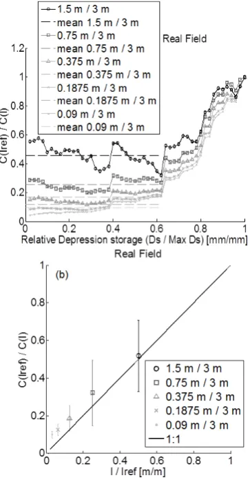
Fig. 15. Real field – scale effect when changing the length: (a) ra-tio of connectivities at different scales as a funcra-tion of the relative depression storage. Horizontal dashed lines correspond to the mean value of the connectivity ratio calculated over the range RDS = 0 to RDS = 0.62. (b) Correlation between the scale ratios and the ratios of connectivities for the first two thirds of the RSC function. Vertical lines = standard deviation. All the plots are 3 m wide.

4.3 Scale effect on overland flow connectivity produced by changing only the length

(12)

0 0.2 0.4 0.6 0.8 1

0 0.2 0.4 0.6 0.8 1 1.2

Relative Depression storage (Ds / Max Ds) [mm/mm]

C(

lref

) /

C

(l)

(a) River type 3 m / 6 m

mean 3 m / 6 m 1.5 m / 6 m mean 1.5 m / 6 m 0.75 m / 6 m mean 0.75 m / 6 m 0.1875 m / 6 m mean 0.1875 m / 6 m 0.375 m / 6 m mean 0.375 m / 6 m

Relative depression storage (Ds / Max Ds) [mm/mm] 0 0.2 0.4 0.6 0.8 1

0 0.2 0.4 0.6 0.8 1

l / lref [m/m]

C(

lref)

/ C(

l)

River type

(b)

3m / 6 m 1.5m / 6 m 0.75m / 6 m 0.375m / 6 m 0.1875m / 6 m 1:1

0 0.2 0.4 0.6 0.8 1

0 0.2 0.4 0.6 0.8 1 1.2

Crater type

C(

lref)

/

C

(l)

(a)

0 0.2 0.4 0.6 0.8 1

0 0.2 0.4 0.6 0.8 1 1.2 1.4

C(

lre

f)

/ C(

l)

(a) Random type

Relative depression storage (Ds / Max Ds) [mm/mm] 0 0.2 0.4 0.6 0.8 1

0 0.2 0.4 0.6 0.8 1

l / lref [m/m]

C(

lre

f)

/ C(

l)

Random type

(b)

0 0.2 0.4 0.6 0.8 1

l / lref [m/m]

C

(lr

ef

) /

C

(l)

Crater type

[image:12.595.111.484.67.539.2]

(b)

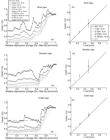
Fig. 16. Synthetic fields – scale effect when changing the length for the river, random and crater microtopographies: (a) ratio of connectivities at different scales as a function of the relative depression storage. Horizontal dashed lines correspond to the mean value of the connectivity ratio calculated over the range RDS = 0 to RDS = 0.5–0.7. (b) Correlation between the scale ratios and the ratios of connectivities for the first two thirds of the RSC function. Vertical lines = standard deviation. All the plots are 6 m wide.

increases rapidly and the separation between the curves pro-gressively decreases until they all meet when the field is com-pletely connected (relative depression storage = 1).

Since for a given scale the ratioC(lref)/C(l)appears to oscillate around a mean value as long as RDS<0.5–0.7, the values ofC(lref)/C(l)for this part of the function were av-eraged and compared to the ratiol/lref, wherelref=3 m for the real field (Fig. 15b) andlref=6 m for the synthetic fields

(Fig. 16b). In this interval of RDS, both ratios show a di-rect correlation, implying that the rate of change of the ratio

C(l)/C(lref) is inversely proportional to the rate of change of the length ratio (l/lref). Since connectivity is the ratio of area connected to the outflow boundary and it increases at the same rate as the length decreases, the size of the area connected (in absolute units, m2) must be approximately the same for all the length scales. This is supported by Fig. 17,

(13)

44 1

2

Figure 17 Surface of the area connected to the outflow boundary, in absolute units (m²), as a 3

function of the relative depression storage, for the four microtopography types. 4

5

0 0.2 0.4 0.6 0.8 1

0 1 2 3 4 5 6 7 8 9

Real Field

S

u

rf

a

c

e

c

o

n

e

c

te

d

[

m

2]

3 m x 0.75 m 3 m x 1.5 m 3 m x 3 m

0 0.2 0.4 0.6 0.8 1

0 5 10 15 20 25 30 35 40

River type

S

u

rf

a

c

e

c

o

n

e

c

te

d

[

m

2]

6 m x 0.75 m 6 m x 1.5 m 6 m x 3 m 6 m x 6 m

0 0.2 0.4 0.6 0.8 1

0 5 10 15 20 25 30 35 40

Random type

S

u

rf

a

c

e

c

o

n

e

c

te

d

[

m

2]

6 m x 0.75 m 6 m x 1.5 m 6 m x 3 m 6 m x 6 m

0 0.2 0.4 0.6 0.8 1

0 5 10 15 20 25 30 35 40

Crater type

S

u

rf

a

c

e

c

o

n

e

c

te

d

[

m

2]

[image:13.595.129.466.67.393.2]

6 m x 0.75 m 6 m x 1.5 m 6 m x 3 m 6 m x 6 m

Fig. 17. Surface of the area connected to the outflow boundary, in absolute units (m2), as a function of the relative depression storage for the four microtopography types.

and can be explained as follows. For the first part of the RSC function, which represents the first stage of the depression filling process, the depressions that are most likely to be al-ready connected are the ones located closest to the bottom boundary. These depressions, which occupy a specific area, behave independently with regard to the rest of the depres-sions, further away from the bottom boundary. This con-nected area keeps the same size independently of the plot length except for plots shorter than this area (Figs. 17 and 2). Therefore, the connectivityC gets higher when decreasing the plot length since the total area of study decreases.

After this first stage of the depression filling process (RDS<0.5–0.7), a quick process of connection of the de-pressions starts and dede-pressions located further from the out-flow boundary get connected. This “jump” or sharp thresh-old in the RSC function, which has been observed in all four microtopographies, is more noticeable for the longer plots (>3 m) (Fig. 17). This is consistent with the percolation the-ory (Berkowitz and Ewing, 1998), whose applicability on overland flow was demonstrated by Darboux et al. (2002a) and Lehman et al. (2007). It relies on the existence of a threshold relationship between rainfall and overland flow,

caused by variations in the storage capacity and connec-tivity. Below a certain threshold, preferential pathways that go from the top to the bottom boundary are still not con-nected and the overland flow remains very low. But when this threshold is exceeded, the pathways become connected and a sharp increase in the overland flow occurs. Applying this concept, the percolation threshold can be calculated as the value of relative depression storage needed to connect the bottom boundary with the top boundary (Table 1). The val-ues obtained for the four microtopography types are slightly higher than the threshold observed in the RSC function. This observed threshold can be assumed to represent the initiation of the connection between the bottom and the top boundary of the plot just before the complete percolation threshold is reached.