www.hydrol-earth-syst-sci.net/16/4467/2012/ doi:10.5194/hess-16-4467-2012
© Author(s) 2012. CC Attribution 3.0 License.
Earth System
Sciences
Exploring the physical controls of regional patterns of flow duration
curves – Part 3: A catchment classification system based on regime
curve indicators
E. Coopersmith1, M. A. Yaeger1, S. Ye2, L. Cheng3, and M. Sivapalan1,2
1Department of Civil and Environmental Engineering, University of Illinois at Urbana-Champaign, Urbana, IL, USA 2Department of Geography, University of Illinois at Urbana-Champaign, Urbana, IL, USA
3Water for a Healthy Country Flagship, CSIRO Land and Water, Canberra, ACT, Australia
Correspondence to: E. Coopersmith ([email protected])
Received: 9 May 2012 – Published in Hydrol. Earth Syst. Sci. Discuss.: 6 June 2012
Revised: 10 September 2012 – Accepted: 5 November 2012 – Published: 26 November 2012
Abstract. Predictions of hydrological responses in ungauged catchments can benefit from a classification scheme that can organize and pool together catchments that exhibit a level of hydrologic similarity, especially similarity in some key variable or signature of interest. Since catchments are com-plex systems with a level of self-organization arising from co-evolution of climate and landscape properties, including vegetation, there is much to be gained from developing a classification system based on a comparative study of a popu-lation of catchments across climatic and landscape gradients. The focus of this paper is on climate seasonality and sea-sonal runoff regime, as characterized by the ensemble mean of within-year variation of climate and runoff. The work on regime behavior is part of an overall study of the physical controls on regional patterns of flow duration curves (FDCs), motivated by the fact that regime behavior leaves a major imprint upon the shape of FDCs, especially the slope of the FDCs. As an exercise in comparative hydrology, the pa-per seeks to assess the regime behavior of 428 catchments from the MOPEX database simultaneously, classifying and regionalizing them into homogeneous or hydrologically sim-ilar groups. A decision tree is developed on the basis of a metric chosen to characterize similarity of regime behavior, using a variant of the Iterative Dichotomiser 3 (ID3) algo-rithm to form a classification tree and associated catchment classes. In this way, several classes of catchments are dis-tinguished, in which the connection between the five catch-ments’ regime behavior and climate and catchment proper-ties becomes clearer. Only four similarity indices are entered
into the algorithm, all of which are obtained from smoothed daily regime curves of climatic variables and runoff. Results demonstrate that climate seasonality plays the most signifi-cant role in the classification of US catchments, with rain-fall timing and climatic aridity index playing somewhat sec-ondary roles in the organization of the catchments. In spite of the tremendous heterogeneity of climate, topography, and runoff behavior across the continental United States, 331 of the 428 catchments studied are seen to fall into only six dom-inant classes.
1 Introduction
Through numerical simulations with a physically based rainfall-runoff model applied to hypothetical catchments, Yokoo and Sivapalan (2011) showed that the FDC of total runoff can be partitioned into two components: the FDC of the surface (or fast) flow and that of subsurface (or slow) flow. This result has been further confirmed by the compre-hensive analysis of the FDCs of some 200 catchments located within the continental United States by Cheng et al. (2012). Yokoo and Sivapalan (2011) further argued that while both the fast and slow flow components are driven by different climate and landscape properties, the FDC of the slow, sub-surface flow component closely resembles and could be more easily reproduced from the catchment’s regime curve. If this is true, then spatial variations of the regime curve, and asso-ciated climatic and landscape controls that result from their interactions, could help explain the regional patterns of the FDCs within the continental United States. So while under-standing of the process controls of the regime behavior is im-portant in its own right, it is also valuable for understanding the controls of the FDC.
Catchments everywhere are highly variable, displaying enormous complexity, with a large number of degrees of free-dom, which makes it very difficult to make general state-ments about their responses. Yet, despite substantial hetero-geneity and the complexity of their responses exhibited by observations, experience with modeling studies and predic-tions indicates that, at the catchment scale, simple models with a small number of parameters can describe the major-ity of catchment responses (Sivapalan et al., 2003). This has encouraged hydrologists to organize and classify catchments into homogeneous or similar groups on the basis of a small number of explanatory variables, as a vehicle towards gener-ating improved understanding and predictions (Dooge, 1986; Bl¨oschl and Sivapalan, 1995; McDonnell and Woods, 2004; Olden et al., 2011). Due to the self-organization of climatic and landscape features arising from their co-evolution, and their impact on multi-scale process interactions and feed-backs, any catchment classification system must be neces-sarily holistic.
One of the pivotal differences between our work and its predecessors is the scope of our classification attempts. For instance, a finely detailed study by Mosley (1981) classi-fied hydrologic responses in 175 small catchments in New Zealand, resulting in narrowly defined characteristics and finely split classes. Ogunkoya (1988) classified 15 catch-ments in Nigeria, but considered lithographic details and other features that may be less appropriate if a classifica-tion scheme is to be broadly applied and minimalist in its information requirements, as is the objective of this work. Burn (1997) applied seasonality metrics to help understand flood frequencies in 59 prairie catchments in central/western Canada chosen specifically because they experience compa-rable climates, and thus all present hydrologic regimes driven by flood events from spring snowmelt. Their results, while useful, do not address the tremendous climatic diversity that
can occur at the continental scale. Recognizing this, Burn and Goel (2000) chose a more diverse assortment of catch-ments in India, using ak-means technique to effectively ex-tract groups of similar catchments. While these catchments exhibited more geographic complexity than the previously discussed studies, this location is still somewhat hydrologi-cally limited. In addition, clustering algorithms of this kind present groups that are similar without specifying the physi-cal drivers that contribute to such similarity – an imperative for deeper understanding of process controls.
Rather than simply examine how quantitative character-istics of catchments in various regions are optimally orga-nized, this analysis also focuses upon why these catchments present the observed climatic and hydrologic characteristics that they do. As mentioned earlier, to understand the physical controls on the FDC, one can classify runoff regimes using empirical runoff regime data, as seen in Haines et al. (1988), where clusters of catchments with similar flow regimes were obtained by minimizing within-group variance of clusters of monthly streamflows. While this procedure does yield quali-tative explanations, they were generated after the fact, rather than as part of the analysis itself. Qualitative insights are strongest as the result of objective, rather than reflective anal-ysis. One way of gaining qualitative insights from an objec-tive process is the use of hydrologic signatures. Wagener et al. (2007) proposed a classification system that is based on similarity of key signatures of catchment runoff response, in-cluding, with decreasing timescale, inter-annual variability, regime curve (i.e., mean within-year variability of runoff), and the flow duration curve (FDC). Taking this idea further, Sawicz et al. (2011) classified catchments located in the east-ern half of the United States, using several catchment-based signatures including the runoff ratio, the slope of a flow du-ration curve, and other streamflow properties. This was fol-lowed by a comparative study of several catchments based on detailed physically based modeling that can account for differences in topography, soil types, geomorphology, and vegetation (Carillo et al., 2011). These studies began investi-gating the physical underpinnings of the groups that emerge from classification – we intend to continue in a similar vein, using simple regime-curve-based features.
With respect to hydrologic, signature-based classification, there has been considerable success in developing similarity measures and catchment classification on the basis of mean annual runoff, expressed in terms of the Budyko curve and the aridity index (Budyko, 1974; Zhang et al., 2001). The fo-cus on the regime curve in this paper is a natural extension to establish the basis for similarity of catchment responses. Whereas the competition between water available and en-ergy available governs similarity at the annual timescale, the shape of the regime curve is governed additionally by the rel-ative timing of precipitation and potential evaporation, and the ability of the landscape to store and release water.
climates using basic information on the variability of precip-itation and temperature (K¨oppen, 1936), and later updated by Peel et al. (2007). The classification of regime behavior presented in this paper can be seen as a precursor to a pos-sible hydrological extension of the K¨oppen-Geiger system towards classification of catchment responses. The K¨oppen-Geiger system is based on the number of months in which average precipitation or average temperature exceeds a given threshold. However, by excluding hydrology from the sys-tem, it fails to distinguish certain catchments that display dif-ferent filtering behaviors. Consider that K¨oppen-Geiger clas-sifies the entire southeastern United States identically. Un-derstanding the distinctions in rainfall/runoff timing allows for more nuanced analysis of the FDC – this was the hypoth-esis raised by Yokoo and Sivapalan (2011) upon which this paper builds.
This paper is the third of a four-part series whose aim is to better understand the physical drivers of observed regional patterns of the FDCs. The first paper, by Cheng et al. (2012), focuses directly on the FDC and approaches the problem em-pirically, while the second (Ye et al., 2012) adopts a top-down modeling approach to explore the process controls of the regime curve and their subsequent relationship to the FDC. The final paper (Yaeger et al., 2012) synthesizes the insights from the different perspectives of the first three papers. The present paper begins with a discussion of hydrologic simi-larity, specifically that of regime behavior. Four key indices that will be used to quantify hydrologic similarity and the reasons for their selection are then presented in Sect. 2. This is followed in Sect. 3 by details of the methodology used to construct the decision tree. Section 4 presents the results of the implementation of the decision tree, while the robustness of the classification tree is verified in Sect. 5. The paper con-cludes with a hydrologic assessment of the catchment clas-sification achieved, including lessons learned and questions left for future work.
2 Similarity of regime behavior
Since the focus of this paper is on catchment regime behav-ior, two catchments will be considered hydrologically sim-ilar if their regime behavior can be deemed simsim-ilar. In this paper, four key similarity indices will be used to characterize the similarity of regime behavior, and are defined and dis-cussed in detail later in this section. These include (i) arid-ity index, a measure of aridarid-ity that, to first order, determines the annual water balance, (ii) a seasonality index that quanti-fies the strength of seasonal variability of precipitation within the year, (iii) the timing (mean date) of precipitation peak within the year, and (iv) the timing (mean date) of runoff peak within the year. Since the climate of the continental United States is such that the seasonal variation of energy (and temperature) is relatively uniform across the country, the timing of precipitation is effectively a measure of the
phase difference between the seasonality of precipitation and potential evaporation. On the other hand, the timing of the runoff peak (especially in relation to precipitation and poten-tial evaporation) captures the mechanisms of storage (in soil water or snow storage) and release (in terms of subsurface drainage or snowmelt). In this sense the similarity indices provide a first-order mapping towards the regional variations in dominant processes highlighted in the parallel study of Ye et al. (2012).
2.1 An example of regime behavior
Figure 1 presents the daily regime curves of precipitation, potential evaporation, and total runoff for a Midwestern-American catchment, located in Kansas. The left image (Fig. 1a) is obtained, using MOPEX daily data from 1948 to 2001 (Sivapalan et al., 2011; Cheng et al., 2012)1, using ensemble averaging by calendar day. While Fig. 1a does pro-vide useful information about the within-year (daily) vari-ability of the chosen variables, for the purpose of catchment classification in this paper, a sliding, 30-day moving average is generated, as shown in Fig. 1b. Equation (1) captures this smoothing:
Pi = i+15
P
i−15
Pi
i+15
P
i−15
(1)
wherePi represents the average precipitation for dayiof the
year; as a point of clarification, this calculation is circular. Many hydrological analyses (K¨oppen, 1936; Haines et al., 1988, and others) deploy monthly regime data to depict sea-sonal patterns of rainfall and runoff. A 30-day moving aver-age achieves this idea of a 30-day window without creating arbitrary monthly boundaries. In classifying catchments on the basis of the daily regime curves of climatic and runoff data, in this paper we will focus upon images like this one (Fig. 1b) for all 428 catchments within the MOPEX database (Duan et al., 2006). The proposed classification scheme will be built around four key indices, each extracted from the smoothed regime curves of the type presented in Fig. 1b. 2.2 Similarity indices used
In the spirit of K¨oppen-Geiger, a key objective of this re-search is the classification of regime behavior using an abso-lute minimum quantity of data, on the basis of four very sim-ple and widely available similarity indices. To estimate these four indicators, three daily time series are required: precipita-tion, potential evaporaprecipita-tion, and total runoff. The first index is the aridity index (Ep/P ), the ratio of annual potential evap-oration to annual precipitation; it measures the competition 1MOPEX data obtained from http://voda.hwr.arizona.edu/
(a)
(b)
Fig. 1. (a) Daily regime curve, and (b) 30-day moving average, Marais des Cygnes River, near Ottawa, Kansas, USA.
between energy available and water available, and is seen as a good first-order indicator of runoff ratio (ratio of annual runoff to annual precipitation). Note that the phase ofEp/P is not addressed because, within the continental US, every catchment’sEp curve peaks within a couple of weeks dur-ing the summer, andEpis very low during winter months; thus the curve’s amplitude is subsumed by the valueEp/P. The seasonality index and maximum day of precipitation are both estimated from the daily precipitation time series. The seasonality index measures the strength of within-year (sea-sonal) variability of precipitation, and is zero if the precipi-tation is uniform throughout the year. The timing of rainfall peaks is a reflection of the phase difference between the tim-ing of the precipitation peak and that of potential evaporation (Milly, 1994), given that, in the continental United States, the timing of potential evaporation’s peak is uniform spatially. Finally, the timing of maximum runoff accounts for the re-sponse of the catchment to the interactions between precipi-tation and potential evaporation. The timing of runoff allows for differences in storage and release processes between dif-ferent regions, owing to distinctions in topography, snowfall, snow storage and melt processes, and also differences in the physiological responses of vegetation. The decisions with re-spect to the four indices are justified in terms of understand-ing the interplay between wettunderstand-ing and dryunderstand-ing, and the timunderstand-ing separating rainfall from runoff, as discussed in Cheng et al and Ye et al. (2012). Within the United States, any three in-dices are insufficient to understand the nuanced behavior of
the catchments we examined, but the addition of a fourth (at least for the vast majority of MOPEX catchments) resolves the discrepancies.
In essence, the four indices represent answers to the fol-lowing four questions:
– “Is this catchment very humid, somewhat humid, tem-perate, somewhat arid, or very arid?”
– “Is rainfall relatively consistent year-round, somewhat seasonally dependent, or highly seasonally dependent?” – “When, during the year, is rainfall greatest?”
– “When, during the year, is streamflow greatest?”
Other variables, such as runoff ratio (Q/P) were consid-ered, but ultimately not adopted because they were correlated with other variables (Ep/P) and failed to improve the quality of classification. Our classification system was reconstructed after the omission of each of the four features to verify that, in fact, all four features are necessary. Further justification of the four features selected is available within the Supplement. With respect to the independence of the four features, sea-sonality and aridity index are almost entirely independent (r2∼0.14). Seasonality and date of max precipitation are fully independent (r2<0.01). Seasonality and date of max runoff are almost entirely independent (r2∼0.14). Aridity index and date of max precipitation are independent (r2∼ 0.05). The same is true for aridity index and date of max runoff (r2∼0.06). Though one might suspect the date of peak precipitation and peak runoff to be related, the r2-value connecting the date of maximum precipitation and the date of maximum runoff is only 0.21. Though there are clusters where the maximum runoff follows the maximum rainfall by a few days or weeks, there are also numerous catchments with virtually constant annual rainfall, yet still characterized by a defined runoff peak. Finally, there are catchments that receive their highest rates of precipitation during fall/winter, then store that water in snowpacks, yielding peak runoff in April, May, or June.
While there are other features that are relevant in under-standing the behavior of a given catchment (proportion of precipitation as snow, etc.), these concepts are included, at least in large part, in the four features chosen. While these four features are sufficient for our purposes, future research may consider adding further indicators to improve specifica-tion within certain regions.
2.2.1 Aridity index: dry or wet?
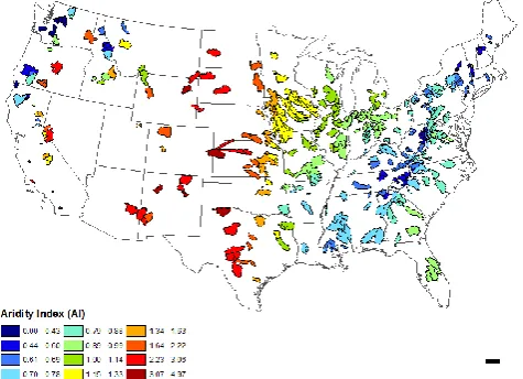
[image:4.595.84.252.61.334.2]rates over the same 365-day period. The aridity index thus measures the competition between energy available and wa-ter available annually:Ep/P >1 for arid (dry) catchments whereasEp/P <1 for humid (wet) catchments.
Figure 2 presents regional patterns of the aridity index for 428 catchments belonging to the MOPEX database. It shows that eastern catchments tend to be largely humid (ex-cept in the south), whereas Midwestern catchments tend to be mostly semi-arid, becoming more arid as they approach the Rocky Mountains and the desert south-west, and becoming humid again in the Pacific Northwest. Essentially one finds systematic east–west (and north–south) trends in the aridity index, contradicted by some outliers in the south-east and north-west.
2.2.2 Seasonality index: is precipitation uniform or periodic?
Figure 1 presented a catchment whose precipitation and also runoff response exhibited significant seasonality, with rain-fall being much higher during the summer than during win-ter months. This is a feature exhibited by a significant num-ber of catchments belonging to the MOPEX database. Poten-tial evaporation is also highly seasonal, although in this case there is very little phase difference between precipitation and potential evaporation. The relative magnitudes of precipita-tion and potential evaporaprecipita-tion are likely to have an impact on runoff regime, and must be accounted for in the classification scheme. Walsh and Lawler (1981) defined a seasonality in-dex for precipitation on the basis of average monthly rainfall values, which in essence is a measure of within-year vari-ance. In this paper we use an adaptation of Walsh and Lawler to accommodate the 365-day smoothed precipitation regime curve as follows:
365
P
i=1
Pi−
365 P
i=1
Pi
365
365
P
i=1
Pi
, (2)
wherePirepresents the value obtained from Eq. (1) The
sea-sonality index helps to distinguish those regions in which precipitation is highly variable seasonally from those in which rainfall is comparatively uniform throughout the year. Figure 3 presents the spatial distribution of the esti-mated seasonality index across the USA. In the eastern part of the country, precipitation is fairly uniform year-round with the exception of three catchments located in southern Florida. Moving westward, the seasonality index tends to in-crease displaying moderate seasonality in the Midwest (mid-continent) and peaking in those catchments near the Pacific. While there are a few catchments that do not follow this trend in the northern Rocky Mountains, the general trend remains consistent.
Fig. 2. Spatial distribution of the aridity index (Ep/P).
2.2.3 Day of peak precipitation: in-phase or out-of-phase with respect to PE?
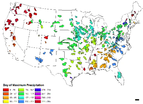
With the seasonality index defining the strength of seasonal variability of precipitation, another key feature is the timing of the maximum precipitation within the year. In this case, the metric we use is the date (from 1 to 365) on which the smoothed precipitation regime curve has its peak. Given that the timing of the peak of potential evaporation is uniform throughout continental United States, the timing of the pre-cipitation peak serves to focus attention to the phase differ-ence between these climate variables, i.e., whether precipita-tion seasonality is in phase with that of potential evaporaprecipita-tion (e.g., precipitation peaks during June or July), is out-of-phase (precipitation peaks during December or January), leading PE somewhat (precipitation peaks during spring months) or lagging PE somewhat (precipitation peaks during fall months). As a side note, it is important that this similar-ity index be estimated from a regime curve obtained with a suitably long moving window to avoid mischaracterizing a catchment. These distinctions are important, since the phase differences between the seasonality of water input and en-ergy input impact storage and release mechanisms, and can thus impact the magnitude and timing of runoff as well.
Figure 4 presents the distribution of the day of maximum precipitation using a circular color coding; i.e., if the day of maximum precipitation happens to fall on 31 December for a catchment, then the similarity index is quite similar to an-other catchment with its precipitation peak falling on 2 Jan-uary, even though the timing index will be “365” for the first catchment and “2” for the second catchment. Although nu-merical values are different, they are actually similar with re-spect to the timing of the precipitation peak. The color coding reflects this similarity.
Fig. 3. Spatial distribution of the seasonality index.
Midwestern regions see precipitation peak in the late spring to early summer, there is much more variability across the continent, creating smaller clusters that are less defined by longitude and latitude alone. The southern Appalachians are quite different from their northern, snowy counterparts; the Pacific coast displays a notable gradient north to south, and several catchments in the monsoon-influenced southwest dis-tinguish themselves from their snowmelt-driven neighbors to the north, and their hurricane-influenced neighbors to the east.
2.2.4 Day of peak runoff: role of catchment storage and release processes
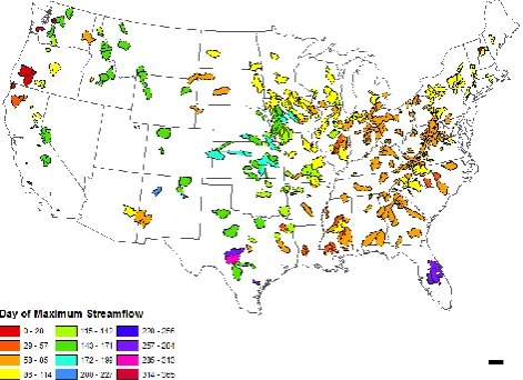
Analogous to the day of peak precipitation, the day of peak runoff (1–365) is the final piece to the classification puz-zle. In this case, the differences between the catchments re-flect not only the magnitude and phase differences between precipitation and potential evaporation, but also the transfor-mations that happen at the land surface (storage and release processes, including below-ground soil and groundwater pro-cesses and above-ground snow storage and snowmelt), as il-lustrated by Milly (1994).
[image:6.595.53.279.64.235.2]The results are presented in Fig. 5, once again using a color coding scheme that is circular (1–365). As with the day of peak precipitation, we observe clusters that are not solely longitude- or latitude-driven, including considerable local variations that may reflect landscape heterogeneity. The Pacific Northwest distinguishes itself due to the out-of-phase relationship between precipitation (peaks during winter) and potential evaporation (peaks during summer). In the Midwest and along the east coast, there is considerable heterogene-ity, and in some cases even adjacent catchments show dif-ferences in runoff timing. Along the Appalachian Mountains in the eastern half of the continent, runoff peaks appear in early spring, presumably driven by melting snow and spring rainfall.
Fig. 4. Spatial patterns of the day of peak precipitation day (1–365).
3 Developing a catchment classification system: decision trees, similarity metrics, and clustering algorithms
3.1 Decision trees for grouping catchments
The goal of this section is to describe the methodology adopted in this paper to “group” catchments exhibiting sim-ilar regime behavior, and separate them from those that are different. Figures 2 through 5 also exhibited certain regional trends across the continental USA with respect to each of the four similarity indices we had considered, and some level of clustering. In the same way, if the regime curves of the type presented in Fig. 1, generated for each of the 428 catchments in the MOPEX database, are superimposed upon a large map of the USA, one could see regional trends, including the emergence of distinct clusters of similar regime behaviors (at least qualitatively). Is there a connection or possible mapping between the former and the latter? Our hypothesis in this pa-per is that a combination of the 4 similarity indices governs the regime behavior and can be the basis of their classifica-tion.
Fig. 5. Day of peak runoff (1–365).
delivers groups without explanation. With this method, as “observers” of the algorithm, we can see what splits occur on what values at what point in the process, allowing us to ask the following: What is the most important, most distin-guishing characteristic for all US catchments? What if we only consider the non-seasonal half? Constructing such trees requires a suitable metric – a mathematical definition of simi-larity (of regime behavior) that can be deployed for any group of catchments – a metric that encompasses the four key in-dices.
3.2 Metric of regime similarity
Each of the four similarity indices, seasonality index (S), the aridity index (A), day of peak precipitation (τp)and
maxi-mum runoff day (τq), shows considerable variability across
the catchments, which can be expressed in terms of a vari-ance measure. ForSthis is straightforward, with the estima-tion of the standard deviaestima-tion obtained from
σS=
v u u u t
n
P
i=1
(Si−µS)2
n−1 (3)
whereSi is the seasonality index for catchmenti,µS is the
its mean over all catchments, andn=428 is the number of catchments. An analogous estimate can be obtained for the standard deviation of the aridity index,σA.
In contrast, forτpandτq, this estimation is not as
straight-forward. This is due to the circularity of the timing of the two peaks (i.e., 1–365), as in the case of four catchments whose values forτpare 361, 364, 359, and 3. To overcome this, we
transformτp andτq into new variables C1andC2, both of which naturally fall between−1 and+1, and overcome the circularity problem.
C1=sin
τp
365·2π
, C2=cos
τp
365·2π
(4)
By estimating σC1 andσC2, the standard deviations of C1,
andC2, respectively, we can then estimate the standard devi-ation ofτp,στP, as follows:
στP =
q σC2
1+σ
2
C2. (5)
The standard deviation ofτq, expressed asστQ, can be
esti-mated in an analogous manner.
In summary, for the four similarity indices outlined, their between-catchment variabilities across the entire MOPEX database of 428 catchments are characterized byσS,σA,στP,
and στQ respectively. To ensure that no one index
over-whelms the others by virtue of its numerical scales, the vari-ance of each index, whether it contains all 428 catchments or a smaller subset of them, is normalized by the four con-stants listed above. For any group ofmcatchments, we define a new quantity,E, the metric of regime similarity associated with that group, as follows:
E=
v u u t
σS,m
σS
2
+
σA,m
σA
2
+
στP,m
στP
2
+ στq,m
στq
!2
. (6)
Essentially, the regime similarity metric,E, is a representa-tive measure of the combined within-group variance of the four similarity indices for any group ofmcatchments, with equal weights attached to each of the similarity indices. 3.3 Clustering algorithm: Iterative Dichotomiser 3
algorithm (ID3)
Classification trees offer a straightforward approach for grouping objects on the basis of similarity or variance mea-sures (Breiman et al., 1984). Such tools are routinely in-cluded in many statistical programming packages (Breiman et al., 1993). The clustering or grouping algorithm used in this paper is the Iterative Dichotomiser 3 (ID3) algorithm de-veloped by Quinlan (1986), which was re-coded as part of this research. This algorithm has found classification appli-cations in forest resource management (Aertsen et al., 2011), crop identification for soil management (Pena-Barragan et al., 2011), mapping of arid rangeland vegetation (Brodley and Freidl, 1997; Lailiberte et al., 2007), and prediction of the failure of business ventures (Li et al., 2010).
By definition, the normalized value of the variance of the entire distribution of any independent variable is equal to unity. Substituting into Eq. (6) to obtain the value ofE of the initial data belonging to 428 catchments yields
E=
q
(1)2+(1)2+(1)2+(1)2= √
4=2. (7)
When all 428 catchments were assessed, although each of the four similarity indices was considered, the best-performing splitting criterion turned out to be a seasonality index of 0.2564. There are 266 catchments with seasonality index val-ues less than 0.2564 and 162 with seasonality indices that ex-ceed 0.2564. The new value of the regime similarity index,
E, is now calculated as follows:
E0=266 ES≤0.2564+162(ES>0.2564) . (8)
In this case,ES≤0.2564denotes the regime similarity metric of the set of catchments, for whichS≤0.2564 (266 in all)
andES>0...2564represents the similarity metric of the set of
catchments for whichS >0. 2564 (162 in all). In each term of Eq. (8), Eq. (6) is now used to estimateEfor only the sub-groups of 266 and 162 respectively. Substituting into Eq. (8) this gives, after the first split,
E0=[266(1.1838)+162(2.1992)]/428=1.5681. (9) This represents the minimum possible value ofEafter one single split. Thus what began with an E-value of 2 has now improved to 1.5681. It is worth noting that one branch, the one with more seasonal catchments, actually displays greater “disorder” than the entire dataset. However, given that 266 of the 428 catchments begin to cluster significantly (i.e.,E= 1.1838), the small increase in the disorder of the remaining 162 is justified.
At this point, the algorithm as described above can be re-peated recursively, locating an optimal split criterion at each node by choosing from one of the four similarity indices, thus branching outward down the tree. Splitting ceases when it is determined that the catchments within a given terminal node are maximally similar – no further splitting will decrease the regime similarity metric significantly, or there is only a sin-gle catchment left at that node (and thusEis zero). In some cases, there are very few catchments left in a given node to be split with an obvious pair of clusters. In such cases, adopting different splitting criteria might yield the same two groups. In these rare cases, a manual choice of splitting is invoked to choose the most appropriate class delineator.
4 Results: what patterns emerge, and where are the largest clusters?
We now present the results of the application of the clus-tering algorithm presented above, describing the breakdown developing at each level of the decision tree. For presenta-tion purposes, depending on the magnitudes of the similarity
indices at which the splits occur, we divide each similarity in-dex into several (3 to 5) distinct and meaningful classes. The combination of these classes then produces the nomenclature we need to describe the catchment classes at each level. 4.1 Nomenclature for catchment classes
The nomenclature we have adopted is letter-based, using up to five letters of the alphabet to characterize the range of val-ues of each of the four similarity indices; these are presented below.
4.1.1 Codes for aridity index
– V= “Very Humid”,Ep/P <∼0.5; – H= “Humid”,∼0.5< Ep/P <∼0.75; – T= “Temperate”,∼0.75< Ep/P <∼1.2; – S= “Somewhat Arid”,∼1.2< Ep/P <∼2; – A= “Arid”,∼2< Ep/P.
4.1.2 Codes for seasonality index
– L= “Low Seasonality”,S <∼0.25;
– I= “Intermediate Seasonality”,∼0.25< S <∼0.5; – X= “eXtreme Seasonality”,∼0.5< S.
4.1.3 Codes for day of precipitation peak
– J= “June”, max rainfall occurs in early or mid-summer (not necessarily in June);
– W= “Winter”, max rainfall occurs in winter (mid-February or March);
– B= “Blizzard”, max rainfall in late November to mid-February;
– P= “Printemps”, max rainfall during spring. 4.1.4 Codes for day of runoff peak
– Q= max runoff during summer months, early June through August;
– F= “Fall/hurricane season”, generally in Septem-ber/October, uncommon (TX & FL);
– M= “Melt”, spring melt usually at a peak in April, May, or early June;
– C= “Cold runoff”, max runoff occurring from early February to before April;
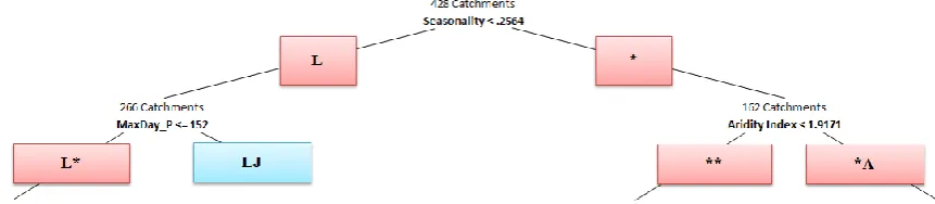
Fig. 6. The top two layers of the classification tree (terminal node shown in blue).
The classes described above can theoretically describe 3×5×4×5=300 different combinations of the similarity in-dices (and associated catchment groupings), although, as will become apparent soon, an overwhelming majority of those combinations will never occur. The nomenclature for these classes was developed after seeing the clusters that emerged. For instance, with respect to the aridity index, there were a few classes whereEp/P was much lower than 0.5, some classes withEp/P greater than 2.5, and three notable group-ings in between. For this reason, five classes were selected. However, with respect to seasonality, in examining groups it became evident that there were catchments with very little seasonality, catchments with extremely high rates of season-ality, and intermediate catchments. Thus, three were chosen. The intention had been to generate as few classes as possible. Indeed we will show that the first six most dominant classes will encompass 331 of the 428 catchments.
4.2 Initial split: top of the classification tree
The classification tree begins with the complete database of 428 MOPEX catchments. As mentioned before, the popula-tion of 428 catchments is split recursively into smaller, more homogeneous groups, being named along the way depending on the value(s) of the similarity indices at play at each split. After the very first split, the dataset is divided into two large clusters, which are not terminal nodes, but rather are inter-mediate nodes, and these are further split into four clusters, and so on. After each split, the resulting pair of clusters be-gins to receive a more detailed code using the letters above, depending on the value of the similarity index that is in play at each split.
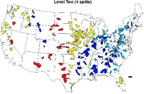
Seasonality turned out to be the single most important fac-tor in creating order in the 428 catchments in the MOPEX database at the first level. Two clusters emerged: one charac-terized by catchments with a low seasonality index (L) and the other characterized by catchments with a “not low” sea-sonality index. This is shown in Fig. 6, with the left branch labeled “L” and the right branch labeled “*” because it could be either an “I” or an “X” type of seasonality. The transfer of the first level split onto a map of the United States makes the classes resulting from the first split easy to understand hydrologically, as seen in Fig. 7.
The results presented in Fig. 7 indicate that the season-ality index, after only one binary split, effectively partitions the continental United States geographically in a meaning-ful way. In the eastern part of the country, rainfall is rela-tively uniform throughout the year, from New England in the northeast, down the Appalachian Mountains to the Ozarks, stretching into the Midwest. Only three eastern catchments in this database, those in Florida, deviate from this pattern, as they see large amounts of rainfall during a warm, hu-mid, hurricane-influenced summer/fall and considerably less during the winter. In the western United States, excluding a handful of catchments in the northern Rocky Mountains, ev-ery catchment displays considerable seasonal variability of precipitation, from the Midwestern catchments characterized by a precipitation that is in phase with potential evapora-tion to the Pacific coast catchments in which the precipita-tion regime is out-of-phase with respect to that of potential evaporation.
The second split criterion, for the lower seasonality, east-ern catchments (colored blue in Fig. 7), is the timing (day) of precipitation peak while for the more seasonal, western catchments, the split criterion becomes the aridity index (see Fig. 3). For less seasonal catchments, the dividing date falls on 1 June; for the more seasonal catchments, the dividing aridity index is roughly 1.9. This leads to four classes, as shown in Fig. 6, one of which (LJ) is a terminal node. The transfer of these four clusters, after two consecutive splits of the original dataset, onto the map of the United States is presented in Fig. 8. The results presented in Fig. 8 show an east-west division based on the seasonality index at the first level; a northeast-southwest split occurs in the eastern (non-seasonal) region via the timing of rainfall, while in the west a split based on aridity index distinguishes the Pacific North-west and the northern MidNorth-west catchments from the remain-ing western catchments.
4.3 Four quadrants of the classification tree
Fig. 7. First split, low seasonality (blue) and higher seasonality (or-ange).
presented. Even here, because of the size of the resulting tree, it is most easily viewed in portions, which we call quadrants, relating to the major clusters formed at the end of the level two splits. In what follows, each quadrant of the classifica-tion tree is presented and discussed in detail.
4.3.1 First quadrant: low seasonality, max precipitation before 1 June
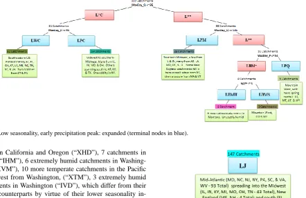
[image:10.595.53.285.64.216.2]Figure 9 presents the expansion of the first quadrant. Six cli-mate regions describe the 119 catchments that comprise this group. The most populous group, “LWC” contains 52 catch-ments, 50 of which are located in the southeastern states. While this terminal grouping has been obtained without the use of the aridity index, using only seasonality and the tim-ings of precipitation and runoff, the 52 catchments all dis-playEp/P <0.87, displaying a tight cluster of humid catch-ments where rainfall and runoff peak in February or March. The second-most populated group is “LPC”, containing 29 catchments from the eastern Midwest. Once again, although the aridity index has not been used as a split criterion to ob-tain this cluster, the 29 catchments have similar Ep/P-values, near or slightly below one. This class is distinguished from LWC by virtue of maximum rainfall occurring later in the spring. A third, well-populated cluster is found in 28 “LPM” catchments located in the southeastern regions of the Mid-west where rainfall and runoff both peak during springtime. The “LBMH” catchment in Montana, which seems unusual for its geography given its low seasonality, and humidity (Ep/P ∼0.67), 3 “LBMS” catchments from Colorado and Montana, which are similar to the LBMH oddity, only con-siderably drier (1.17< Ep/P <1.66), and 6 “LPQ” catch-ments, also from the mountain west (Wyoming) where rain-fall peaks in the spring instead of the winter, round out this quadrant.
Fig. 8. Second split: low seasonality and earlier precipitation peak (dark blue), low seasonality and later precipitation peak (light blue), higher seasonality and non-arid (yellow), higher seasonality and arid (red).
4.3.2 Second quadrant: low seasonality, max precipitation after 1 June
This quadrant becomes fully organized with only two cri-teria for splitting, leaving 147 catchments which all carry the “LJ” designation. Although the maximum date on which runoff occurs is not used to create this class, 145 of the 147 catchments observe maximum runoff between mid-February and late April (the remaining two peaks occur in the first week of May). In fact, 124 of the 147 catchments peak be-tween the second week of March and the first week of April. Furthermore, although once again the aridity index is not used to generate this cluster, all 65 catchments fall between
Ep/P ∼0.5 andEp/P ∼1.05. This class of catchments de-fines the mid-Atlantic and Appalachian regions of the United States, extending into the eastern Midwest. This quadrant of the tree, albeit expressed as a single node, is illustrated in Fig. 10.
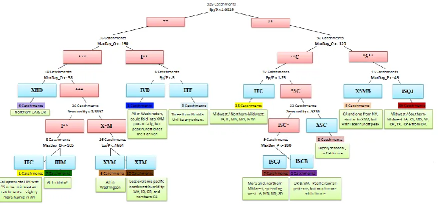
4.3.3 Third quadrant: higher seasonality, non-arid
Fig. 9. Low seasonality, early precipitation peak: expanded (terminal nodes in blue).
northern California and Oregon (“XHD”), 7 catchments in Idaho (“IHM”), 6 extremely humid catchments in Washing-ton (“XVM”), 10 more temperate catchments in the Pacific Northwest from Washington, (“XTM”), 3 extremely humid catchments in Washington (“IVD”), which differ from their XVM counterparts by virtue of their lower seasonality in-dex, and winter runoff peak, 3 Floridian catchments (“ITF”), which are truly unlike any others in the United States, 7 drier Midwestern catchments with early runoff peaks (“ISCJ”), 2 drier Pacific northwestern catchments (“ISCB”), and 3 drier southern Californian catchments (“XSC”), and 6 drier south-ern Californian/Nevadan catchments with later runoff peaks (“XSMB”).
The terminal nodes in the third quadrant contain 10 or fewer catchments, describing certain niche climates of United States. These mini-clusters often describe several catchments that are very similar to each other, but quite dif-ferent from their neighbors.
4.3.4 Fourth quadrant: higher seasonality, arid
In this final quadrant, the 34 remaining catchments are fur-ther divided into five terminal nodes. The most common classification (“IAQ”) contains 16 catchments, a miscella-neous assortment of the country’s most arid locations, in-cluding 10 from the southwest, 5 from the Midwest, and one remarkably arid catchment in Wyoming (the moun-tain west). The remaining clusters consist of three Cali-fornian catchments that represent the driest American Pa-cific climates (“XADB”), the northern Midwestern “bad-lands”, six extremely arid catchments in Nebraska and North and South Dakota (“XACJ”), a cluster of seven arid south-western catchments, one oddity in the Pacific Northwest, (“IACJ”), shielded from the Pacific coast by the Cascade Mountains, and three arid catchments in Texas characterized by runoff peaks occurring as late as the fourth week of Octo-ber (“IAF”). Figure 12 presents the final quadrant.
Fig. 10. Low seasonality, late precipitation peak: expanded (termi-nal node).
4.4 Summary of the resulting catchment classification and the largest six classes
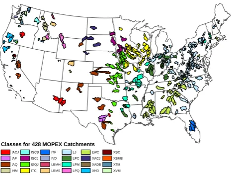
In total, the classification tree yielded 24 terminal nodes, de-picting 24 distinct classes according to the criteria we have used. The geographic representation of these 24 classes on a map of the continental United States is presented in Fig. 13, revealing distinct regional associations of many of the major catchment classes.
Fig. 11. Higher seasonality, non-arid: expanded (terminal nodes in blue).
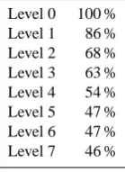
46.5 %. Considering that these groups comprise 77 % of the database, this is quite encouraging, as these clusters contain much less than half of the variance of the original dataset using very simple indices.
Three of the largest six classes are found within the first quadrant (LWC, LPC, and LPM). The catchments belonging to these three classes are characterized by limited seasonal-ity, and are essentially catchments with pre-spring maximum rainfall and runoff (LWC), catchments with pre-spring peak runoff, but mid-spring maximum rainfall (LPC) and catch-ments with springtime rainfall and runoff peaks (LPM). The entire set of catchments in the second quadrant (belonging to the terminal LJ class) is clearly the fourth member of the largest six classes. These catchments display limited sea-sonality, humid climates, peak runoff during the springtime (likely melt-driven from the Appalachian mountain range), and peak rainfall during the summertime. The final two mem-bers of the largest six are found in the third quadrant: ISQJ and ITC (and none of the classes in the fourth quadrant falls within the largest six). The two Midwestern classes, ISQJ and ITC, both contain catchments with rainfall that is in phase with potential evaporation. However, the ISQJ catchments are notably more arid, with Ep/P averaging roughly 1.5, as opposed to an average of roughly 1 for ITC. As a result of the more temperate climate, the ITC group displays peak runoff during early spring, when stored water from winter has thawed. On the other hand, ISQJ, characterized by drier soils, shows its runoff peak in late May or June, at the same time as its precipitation peak.
4.5 Robustness of classification: recurrent, dominant clusters
When classification systems are generated using recursive, splitting algorithms (those that minimize variance at each stage without concern for future splits), there is a tendency to over-fit one’s data. Although variance is minimized at ev-ery stage, ensuring that we do not split a group of catch-ments without purpose, caution is required to prevent fitting the noise inherent in the dataset rather than true patterns. To this end, the same algorithm was applied to a 197-catchment subset of the larger, 428-catchment dataset. These 197 catch-ments were chosen due to their comparatively richer datasets (fewer missing days, more complete years, etc.) and form the dataset that has been employed by Ye et al. (2012), Cheng et al. (2012), and Yaeger et al. (2012) in the accompanying pa-pers that are all focused on exploring the physical controls of the FDCs from different perspectives.
Fig. 12. Higher seasonality, arid: expanded (terminal nodes in blue).
Classes for 428 MOPEX Catchments
IACJ IAF IAQ IHM
ISCB ISCJ ISQJ ITC
ITF IVD LBMH LBMS
LJ LPC LPM LPQ
LWC XACJ XADB XHD
[image:13.595.310.547.272.417.2]XSC XSMB XTM XVM
Fig. 13. All classes.
[image:13.595.51.286.273.450.2]The second quadrant of the 197-catchment tree, like the 428-catchment tree, contains the single class LJ, now com-posed of 65 catchments rather than 147. The remaining two quadrants also show some differences, this likely resulting from the nature of the dataset. Unfortunately, given the chal-lenges associated with data gathering in more arid catch-ments, many of the catchments characterized by substantial missing data are found in the nation’s more arid locations. As a result, the 428-catchment tree contains a much higher proportion of arid catchments (thus, the second split criterion for more seasonal catchments isEp/P ). Conversely, the 197-catchment tree contains a smaller proportion of arid catch-ments and, thus, splits on the maximum day of precipitation to define its third and fourth quadrants. Despite this, the two most common classes on this side of the 428-catchment tree (ISQJ – 39 and ITC – 36) still find their parallels in the 197-catchment tree (ISQJ – 15 and “IJTC” – 20). The remaining, less common groups do display some overlap, although in this case differences appear simply because certain groups
Fig. 14. Clusters of runoff regimes.
are not represented at all in the 197-catchment subset, or find themselves folded into other classes. Despite these minor dis-tinctions, once again, the nearly identical largest six classes again define over 70 % of all catchments and the tree’s gen-eral structure remains intact. This demonstrates that not only is the classification system intuitively satisfying in its sim-plicity, but is robust to alterations in the dataset.
Table 1. Decreasing FDC variance (layer-by-layer down the tree).
Level 0 100 % Level 1 86 % Level 2 68 % Level 3 63 % Level 4 54 % Level 5 47 % Level 6 47 % Level 7 46 %
classification tree. In other words, not only are the four key indices being grouped effectively, but the FDCs of the con-stituent groups are well-organized as well. More detailed dis-cussions of this connection and its relationship to other find-ings from the first two papers of this series can be found in Yaeger et al. (2012).
5 Conclusions
This paper has presented the application of a clustering al-gorithm (i.e., Iterative Dichotomiser 3, or ID3 alal-gorithm) for classifying catchments across the continental United States with respect to their climatic seasonality and regime behav-ior (i.e., mean within-year variation of runoff). The classifi-cation was achieved by assessing the catchments in terms of a metric of regime similarity,E, which is a composite measure estimated on the basis of the magnitudes of four similarity indices: (i) a seasonality index of precipitation, (ii) aridity index, (iii) timing of maximum precipitation, and (iv) timing of maximum runoff. The clustering algorithm was applied to 428 catchments across the continental United States belong-ing to the MOPEX dataset.
The clustering algorithm identified 24 distinct classes. Even though the classification was achieved with just four numbers from each catchment (similarity indices), and only the max date of the runoff regime curve was used, the regime behavior for each of the classes showed distinct differences between classes and strong similarity within. This confirms the power of the simple classification scheme for predicting regime behavior across the continental United States, subject to the limitations of the geographical extent of the dataset and coverage across the country. Considering that three of the four indices used to construct the classification tree are based upon climate, it comes as no surprise that climate’s impact is readily apparent. Just as K¨oppen-Geiger delineated the na-tion into clusters of climatic similarity a century ago, climate still dominates the hydrologic landscape, creating distinct, hydrologically similar clusters.
The resulting classes also display strong regional asso-ciations and patterns, which is very valuable to further ex-plore the climatic and landscape controls underlying the re-sulting catchment classes. Whether the final group is IHM,
with seven catchments all located in the state of Idaho, or ITF, with three catchments all located in Florida, or IAF, with three catchments located in one region of Texas, these groups are not only numerically similar, but geographically contigu-ous as well in many cases.
Despite the enormous heterogeneity of catchments rep-resented in the MOPEX dataset, just six classes accounted for over 77 % of the catchments. The classification system is found to be robust, producing the same recurring six clusters even with a smaller subset of the full dataset. Each of the re-curring, dominant six classes displays distinct characteristics that suggest their own set of hydrologic drivers. In the Mid-west, the aridity index determines whether runoff is driven by the spring thaw of water frozen in soil storage (ITC) or by the arrival of summer rains (ISQJ). In the south-east, runoff tim-ing in late winter (LWC and LPC) or early sprtim-ing is governed by the temperatures in and around the Appalachian Moun-tains. In the north-east, spring runoff is likely the result of melting of snow (LJ). In the area in which the southeastern United States merges with the Midwest, seasonality begins to appear strongly, and runoff is driven by springtime rainfall (LPM). In addition to these largest six clusters, other smaller, niche climates display distinct behaviors. From the monsoon-driven southwest (XACJ), where precipitation occurs mainly in a narrow band of summer months, to the extremely humid Pacific Northwest, where runoff peaks are driven by extreme winter rainfall (IVD) or the melting of snowcaps in the spring (XVM), the United States exhibits a tremendously heteroge-neous group of catchments.
The analyses presented in this paper have identified catch-ment groupings that are similar in terms of their runoff regime. What makes them similar? Their regime curves cer-tainly suggest as much, but does that imply similar dominant processes? The accompanying paper by Ye et al. (2012) ex-plores their regime behavior from a process perspective, by adopting a top-down modeling approach. Is there a recogniz-able mapping between the catchment classification found in this paper and the classification of dominant processes high-lighted in Ye et al. (2012)? Furthermore, this paper has been motivated by our quest to explore the physical controls of the flow duration curve (FDC), considering that the regime curve provides a major connective tissue between the high flow and low flow ends of the FDC. Cheng et al. (2012) presented an empirical analysis of the regional patterns of FDCs across the continental United States and their physical controls. Is there a connection between the regional groupings of catchments based on the regime curve and regional patterns of variation of the FDCs? The accompanying synthesis paper by Yaeger et al. (2012) addresses these questions through cross com-parisons between the results of each of these three studies to draw general conclusions about the physical and process con-trols of the regime curve and the flow duration curve, helping to discover not only which catchments are similar, but also
Finally, it is important to acknowledge the limitations in-herent in the classification system presented. Although the continental United States represents a diverse and rich ar-ray of climate conditions and landscape features, it is nat-ural that it does not contain every conceivable combination of climate and landscapes. It may very well be the case that such climates exist on other continents. It is to be hoped that future efforts will integrate global climate data into an en-hanced tree, duplicating this work on a larger, multi-national scale. Secondly, while the classification system classified 428 gauged catchments (including information on runoff timing) into distinct classes, without a further effort to incorporate catchment or landscape features that impact runoff genera-tion, especially runoff timing, application to ungauged catch-ments is not feasible. This calls for further research that will overcome this major limitation of this study.
Supplementary material related to this article is
available online at: http://www.hydrol-earth-syst-sci.net/ 16/4467/2012/hess-16-4467-2012-supplement.pdf.
Acknowledgements. The work presented in this paper was carried
out as part of the NSF-funded project “Water Cycle Dynamics in a Changing Environment: Advancing Hydrologic Science through Synthesis” (NSF grant EAR-0636043, M. Sivapalan, PI), and also the NSF project “Understanding the Hydrologic Implications of Landscape Structure and Climate – Toward a Unifying Framework of Watershed Similarity” (NSF Grant EAR-0635998, T. Wagener, PI). Special thanks are owed to Matej Durcik of SAHRA (Univer-sity of Arizona) for providing the version of the MOPEX dataset used in this study. We would like to thank Ross Woods and the other reviewers for their constructive criticism and insight – the paper is unquestionably stronger as a result.
Edited by: P. Claps
References
Aertsen, W., Kint, V., Van Orshoven, J., and Muys, B.: Evaluation of modeling techniques for forest site productivity prediction in contrasting ecoregions using stochastic multi-criteria acceptabil-ity analysis (SMAA), Env. Modell. Softw., 26, 929–937, 2011. Bl¨oschl, G. and Sivapalan, M.: Scale issue in hydrological modeling
– a review, Hydrol. Process., 9, 251–290, 1995.
Breiman, L., Friedman, J., Olshen, R., and Stone, C.: Classification and Regression Trees, Wadsworth International Group, Belmont, CA, 1984.
Breiman, L., Friedman, J., Olshen, R., and Stone, C.: Classification and Regression Trees, Chapman and Hall, Boca Raton, 1993. Brodley, C. and Freidl, M.: Decision tree classification of land cover
from remotely sensed data, Remote Sens. Environ., 61, 399–409, 1997.
Budyko, M.: Climate and Life, Academic, New York, 1974.
Burn, D. H.: Catchment similarity for regional flood frequency analysis using seasonality measures, J. Hydrol., 202, 212–230, doi:10.1016/s0022-1694(97)00068-1, 1997.
Burn, D. H. and Goel, N. K.: The formation of groups for re-gional flood frequency analysis, Hydrolog. Sci. J., 45, 97–112, doi:10.1080/02626660009492308, 2000.
Carrillo, G., Troch, P. A., Sivapalan, M., Wagener, T., Harman, C., and Sawicz, K.: Catchment classification: hydrological analysis of catchment behavior through process-based modeling along a climate gradient, Hydrol. Earth Syst. Sci., 15, 3411–3430, doi:10.5194/hess-15-3411-2011, 2011.
Cheng, L., Yaeger, M., Viglione, A., Coopersmith, E., Ye, S., and Sivapalan, M.: Exploring the physical controls of re-gional patterns of flow duration curves – Part 1: Insights from statistical analyses, Hydrol. Earth Syst. Sci., 16, 4435–4446, doi:10.5194/hess-16-4435-2012, 2012.
Dooge, J.: Looking for hydrologic laws, Water Resour. Res., 22, 46S–58S, 1986.
Duan, Q., Schaake, J., Andr´eassian, V., Franks, S., Goteti, G., Gupta, H., Gusev, Y., Habets, F., Hall, A., Hay, L., Hogue, T., Huang, M., Leavesley, G., Liang, X., Nasonova, O., Noilhan, J., Oudin, L., Sorooshian, S., Wagener, T., and Wood, E.: Model Pa-rameter Estimation Experiment (MOPEX): An overview of sci-ence strategy and major results from the second and third work-shops, J. Hydrol., 320, 3–17, 2006.
Haines, A. T., Finlayson, B. L., and McMahon, T. A.: A global clas-sification of river Regimes, Appl. Geogr., 8, 255–272, 1988. K¨oppen, W.: Das Geographisca System der Klimate, in: Handbuch
der Klimatologie, edited by: K¨oppen, W. and Geiger, G., 1. C. Gebr., Borntraeger, 1–44, 1936.
Lailiberte, A., Fredrickson, E., and Rango, A.: Combining decision trees with hierarchical object-oriented image analysis for map-ping arid rangelands, Photogramm. Eng. Rem. S., 73, 197–207, 2007.
Li, H., Sun, J., and Wu, J.: Predicting business failure using classifi-cation and regression tree: An empirical comparison with pop-ular classical statistical methods and top classification mining methods, Expert Syst. Appl., 37, 5895–5904, 2010.
McDonnell, J. and Woods, R.: On the need for catchment classifi-cation, J. Hydrol., 299, 2–3, 2004.
Milly, P.: Climate, soil water storage, and the average water balance, Water Resour. Res., 30, 2143–2156, 1994.
Mosley, M. P.: Delimitation of New Zealand hydrologic regions, J. Hydrol., 49, 173–192, doi:10.1016/0022-1694(81)90211-0, 1981.
Ogunkoya, O. O.: Towards a delimitation of southwestern Nigeria into hydrological regions, J. Hydrol., 99, 165–177, doi:10.1016/0022-1694(88)90085-6, 1988.
Olden, J., Kennard, M., and Pusey, B.: A framework for hydrologic classification with a review of methodologies and applications in ecohydrology, Ecohydrology, 5, 503–518, 2012.
Quinlan, J.: Induction of Decision Trees, Mach. Learn., 1, 81–106, 1986.
Sawicz, K., Wagener, T., Sivapalan, M., Troch, P. A., and Carrillo, G.: Catchment classification: empirical analysis of hydrologic similarity based on catchment function in the eastern USA, Hy-drol. Earth Syst. Sci., 15, 2895–2911, doi:10.5194/hess-15-2895-2011, 2011.
Sivapalan, M., Takeuchi, K., Franks, S., Gupta, V., Karambiri, H., Lakshmi, V., Liang, X., McDonnell, J., Menidiondo, E., O’Connell, P., Oki, T., Pomeroy, J., Schertzer, D., Uhlenbrook, S., and Zehe E.: IAHS decade on predictions in Ungauged Basins. (PUB), 2003–2012, Shaping an exciting future for the hydrological sciences, Hydrolog. Sci. J., 48, 857–880, 2003. Sivapalan, M., Yaeger, M., Harman, C., Xu, X., and Troch, P.:
Func-tional model of water balance variability at the catchment scale: 1. Evidence of hydrologic similarity and space-time symmetry, Water Resour. Res., 47, W02522, doi:10.1029/2010WR009568, 2011.
Wagener, T., Sivapalan, M., Troch, P., and Woods, R.: Catchment classification and hydrologic similarity, Geog. Comp., 1/4, 901– 931, 2007.
Walsh, R. and Lawler, D.: Rainfall seasonality: description, spatial patterns and change through time (British Isles, Africa), Weather, 36, 201–208, 1981.
Yaeger, M., Coopersmith, E., Ye, S., Cheng, L., Viglione, A., and Sivapalan, M.: Exploring the physical controls of regional pat-terns of flow duration curves – Part 4: A synthesis of empiri-cal analysis, process modeling and catchment classification, Hy-drol. Earth Syst. Sci., 16, 4483–4498, doi:10.5194/hess-16-4483-2012, 2012.
Ye, S., Yaeger, M., Coopersmith, E., Cheng, L., and Sivapalan, M.: Exploring the physical controls of regional patterns of flow du-ration curves – Part 2: Role of seasonality, the regime curve, and associated process controls, Hydrol. Earth Syst. Sci., 16, 4447– 4465, doi:10.5194/hess-16-4447-2012, 2012.
Yokoo, Y. and Sivapalan, M.: Towards reconstruction of the flow duration curve: development of a conceptual framework with a physical basis, Hydrol. Earth Syst. Sci., 15, 2805–2819, doi:10.5194/hess-15-2805-2011, 2011.