Multivariate statistical methods for fault detection and classification

(1)

Multivariate Statistical Methods for Fault

Detection and Classification

William Richard Southern,

BEng(Hons), MSc.,

A thesis submitted to the University of Dublin in partial fulfilment of the requirements for the degree of

Doctor in Philosophy

Department of Mechanical & Manufacturing Engineering, Trinity College Dublin,

(2)

(3)

Declaration

I declare that I am the sole author of this thesis and that all the work presented in it, unless otherwise referenced, is my own. I also declare that this work has not been submitted, in whole or in part, to any other university or college for any degree or other qualification.

I authorise the library of Trinity College Dublin to lend this thesis.

William Richard Southern

(4)

Acknowledgements

I wish to offer my thanks to Peter Twigg who helped me at the start of my work. After his move to Manchester, I am indebted to Craig Meskell for his help, advice and general banter throughout and help during the write up.

Throughout my period in Trinity College, I have met a tremendous amount of people. There was a strong communal postgraduate idealogy, and I am glad to have been part of it. Although I would like to mention all acquaintances space precludes this so I wish to extend a thanks to all for the times had in TCD.

The oldest crew of Adriele, Alex, John B, and the ‘Murphs’ are still around and kicking. Seosamh is flying planes and setting a trend of bankrupting small airlines!. Thanks to all in my old office, Mary, Kevin, John G, Laoise, Danny, John V, Paul and John T. Mustard gets a special mention here also. Thanks to Orla in Fluids for being in such good form throughout. George, Laura and Oran too. Thanks to Damien for trying (and miserably failing!) to keep in rounds with me, for his input into mp3 encoding and for his interest into bike related things. A kind thank you is also extended to all staff members of the department during my time there.

The work would have been near impossible without the support and help of my family. My Father Peter, Mother Lorna, Sisters Sonya, Amanda, Kate and my Grandmother Nancy always offered encouragement and support when it was needed and I thank them all.

(5)

Presentations and publications

resulting from this study

W.R. Southern,‘Preliminary Application of Principal Components Analy-sis to a Microchip Test Process for Mixed Signal/Radio Frequency Components’, Advances in Process Analytics and Control Technology (APACT) 2003 Conference, York.

W.R. Southern,‘Multivariate Statistical Process Control for Fault Detec-tion using Principal Component Analysis’, Advances in Process Analytics and Control Technology (APACT) 2004 Conference, Bath.

(6)

List of Figures

1.1 Total Quality Management model (Oakland (1999)) . . . 3

2.1 Definition of a process . . . 13

2.2 A normal distribution . . . 18

2.3 A variable control chart . . . 21

2.4 Control ellipsoids . . . 24

3.1 d- dimensional Euclidean space Rd _{. . . .} ₃₀

3.2 Feature space mapping . . . 30

3.3 Data representation in R2 _{. . . .} ₃₁

3.4 Voronoi tesselation in R2 _{. . . .} ₃₆

3.5 Cluster dendrogram . . . 37

3.6 Bivariate control region . . . 46

3.7 A principal component model . . . 47

4.1 Decision tree representation of weather data, Quinlan (1986) . . . 58

4.2 Binary attribute test conditions . . . 60

4.3 Nominal attribute multiway split test condition . . . 60

4.4 Nominal attribute binary split test condition . . . 60

4.5 Test conditions for a continuous attribute . . . 61

4.6 Entropy function of a boolean classification . . . 63

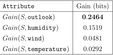
4.7 Information gain for the outlook attribute . . . 65

5.1 A monitoring parallel-coord plot . . . 71

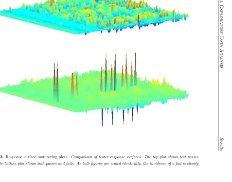
5.2 Response surface monitoring plots . . . 72

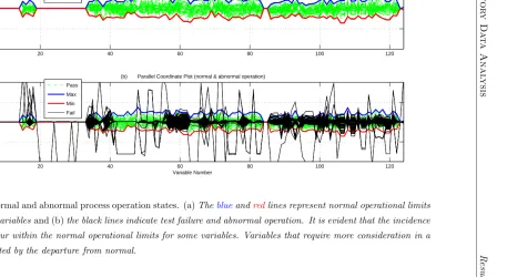
5.3 Normal and abnormal process operation . . . 74

(10)

LIST OF FIGURES LIST OF FIGURES

5.5 Parallel-coord plot . . . 77

5.6 Variable scaling in parallel-coords . . . 79

5.7 Summary parallel coordinate plot . . . 80

5.8 Similarity of tester performance . . . 81

5.9 Combined scree and RMSECV plot . . . 87

5.10 Cumulative variance and eigenvalue plot . . . 88

5.11 NOC score plot . . . 89

5.12 Batch data and NOC model . . . 90

5.13 T2 _and _Q _{multivariate fault indices . . . .} ₉₂

5.14 Contribution plot . . . 94

5.15 Test matrix plot . . . 97

5.16 Combination of fails . . . 98

5.17 Sample decision tree . . . 100

5.18 Batch data decision tree . . . 102

6.1 Known good operation cluster dendrogram . . . 110

6.2 Normal process data cluster dendrogram . . . 111

6.3 Cluster dendrogram including class labels . . . 112

6.4 Normal process parallel-coord plot . . . 115

6.5 Abnormal process parallel-coord plot . . . 116

6.6 Fault detection parallel-coord plots . . . 117

6.7 Fault detection parallel-coord plot (rescaled) . . . 118

6.8 Fault detection parallel-coord plot (rescaled) . . . 118

6.9 Response surface plot with mixed data . . . 119

6.10 PC score plot . . . 126

6.11 PC loading plot . . . 127

6.12 PC1-PC2 score & loading plots . . . 128

6.13 Biplot of PC scores & loadings . . . 129

6.14 PC1-PC2-PC3 score & loadings plot . . . 129

6.15 PC1-PC2-PC3 NOC ellipsoid . . . 130

6.16 PC1-PC2-PC3 NOC ellipsoid with new batch scores . . . 130

6.17 Multivariate detection indices . . . 131

6.18 Multivariate detection indices (rescaled) . . . 131

(11)

LIST OF FIGURES LIST OF FIGURES

6.20 Q contribution plots for sample 21 & 12 . . . 133

B.1 PCA model variance . . . 153

(12)

List of Tables

1.1 Product and process variation . . . 4

2.1 A history of quality . . . 10

2.2 The eleven dimensions of process quality . . . 14

2.3 The eight dimensions of product quality . . . 15

2.4 Decisions in hypothesis testing . . . 17

2.5 The normal distribution with σ levels . . . 18

4.1 Weather data from Quinlan (1993). . . 55

4.2 1R evaluation of attributes . . . 56

4.3 Top-Down Induction of Decision Trees (TDIDT) . . . 62

4.4 Class membership and entropy from Figure 4.6 . . . 63

4.5 Information gain for all 4 attributes . . . 65

4.6 Summary confusion matrix . . . 67

5.1 NOC model flowchart . . . 85

5.2 Fault identification . . . 96

5.3 Classifier confusion matrix . . . 103

5.4 Summary confusion matrix . . . 103

5.5 Batch 1 confusion matrix . . . 103

5.9 Tester HP004 confusion matrix . . . 105

(13)

Acronyms

1R OneRule

DIB Device Interface Board DUT Device Under Test

EDA Exploratory Data Analysis

EWMA Exponentially Weighted Moving Average FDI Fault Detection and Isolation

FPY First PassYield JIT Just In Time

KDD KnowledgeDiscovery in Databases MSPC MultivariateStatistical Process Control MSQC MultivariateStatistical Quality Control

MSRF Mixed Signal and Radio Frequency NOC NormalOperating Condition

PC Principal Component

PCA Principal Component Analysis PDF Probability Density Function PQKB Process Quality Knowledge Base

QFD Quality Function Deployment QI Quality Improvement

SPC Statistical Process Control STDF Standard Test Data Format

(14)

Nomenclature

x Scalar

x Vector

X Matrix

xT _Transpose

X−1 _Inverse

α Probability of type I error β Probability of type II error Z Standard normal variate

x Mean value of x

µ Mean

σ2 _Variance

P

Covariance matrix

m Estimated mean

s2 Estimated variance

S Estimated covariance matrix

N(µ, σ2) Univariate normal distribution with mean µand variance σ2

λ Eigenvalue

et Random noise, error trace(S) The trace of matrix S

T2 _{Hotelling’s} _T2 _metric

(15)

Rd _d_{- dimensional Euclidean space}

Z PCA transform variable

X PCA decomposition

T PCA score matrix

P PCA loading matrix

I Identity matrix

Qα Squared prediction error critical value H(S) Entropy of S

(16)

Abstract

With increased competition in the market place, it is essential that product qual-ity and process performance are consistently competitive. Statistical Process Control (SPC) strives to differentiate between stochastic and assignable causes of variation.

This work outlines multivariate methods used for fault detection and classifi-cation in a high volume semiconductor device batch testing process. The routine capture of large quantities of test information and storage of historical results to databases occurs in most all processes. Subsequent data analysis and modelling is required for process monitoring, fault detection and classification.

Traditional exploratory methods of clustering and parallel coordinate analysis (parallel-coord) plots are used to demonstrate process contributions and diag-nose out of control variables. They also serve as a low level monitoring scheme for process operatives and technicians. Principal Component Analysis (PCA) is applied to the semiconductor device batch test data as a dimension reduction method in order to represent the process through a reduced set of uncorrelated variables. The application of PCA tomixed-mode data, (i.e. analogue and digital variables), and the construction of a Normal Operating Condition (NOC) model is shown to offer fault detection and classification capabilities.

Supervised learning through decision tree induction is implemented with the batch test data for the purpose of fault classification. Use of the C4.5 tree induc-tion algorithm is evaluated. Results for this nontradiinduc-tional exploratory method are presented through confusion matrices.

(17)

Chapter 1 Introduction

1.1 Quality Improvement

(18)

1.2. _{Industrial Application} _Introduction It is difficult to encapsulate the differences that effectively discriminate processes and products of bad quality with processes and products of good quality. Statis-tical Quality Control (SQC), is infact a subset of a higher level philosophy known as Total Quality Management (TQM). This philosophy is expanded upon in table 2.1.1, but suffice it to say that TQM is essentially a framework of collective ideas, a synergistic set of ideals that spreads across an entire organisation. Caulcutt (1995) suggests that although the ideas that define TQM are well established, proper application of the principles result in a more coherent business.

There are a number of key buzzwords and acronyms used frequently within quality circles. Where one company is interested in implementing SQC, another may want Statistical Process Control (SPC). There is tremendous talk of TQM, Quality Function Deployment (QFD), Just-in-Time methodologies (JIT) and World Class Manufacturing (WCM). Although there is a link between quality and productivity, and hence profitability, any improvement requires an organisa-tion or business to fully comprehend their processes and products needs. Two main components that dictate the success of these efforts are a systematic reduc-tion in variability and a focus on statistical methods for process (and product) improvement. Clearly from this, it is difficult to succinctly define a TQM frame-work but in general it is concerned with people, processes and performance.

1.2 Industrial Application

In the semiconductor industry, success is a function of a product being unveiled swiftly and in accordance to market demands. In principle, this success is influ-enced by:

• Wafer defects

• Contamination

• IC manufacturing defects

• Design errors

• Handling problems

(19)

1.2. _{Industrial Application} _Introduction

Teams

Systems Tools

C

ustomer

S

upplier

Process

CU LT

UR E

C O

M M

U N

IC A

T IO

N

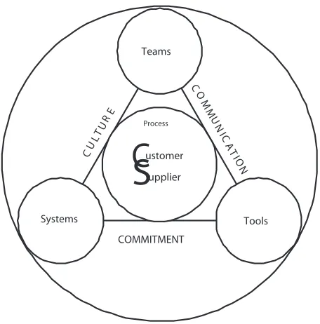
[image:19.612.209.437.57.288.2]

COMMITMENT

Figure 1.1. Total Quality Management model (Oakland (1999))

• External influences

• Process variations

• Product variations

A systematic long term goal for this work was an improvement in the yield of the devices under test (DUT), specifically for First-Pass Yield, (FPY). Improvement in this area could result in positive knock on effects such as reducing re-test batches, batches on hold, scrappage and being able to increase tester capacity. The old adage ‘time is money’ is truly relevant when it comes to the testing of electronic components.

(20)

1.2. _{Industrial Application} _Introduction

Product Attributes Process Attributes

Site-to-Site Wafer-to-Wafer Socket-to-Socket

Lot-to-Lot Picker-to-Picker

Batch-to-Batch DIB-to-DIB

DUT-to-DUT Handler-to-Handler

Tester-to-Tester

Table 1.1. Product and process variation. Some common attributes that

constitute variation (both product and process). This table gives an insight

to some of the variation sources in the testing process.

distributions, pareto of failures, cross platform correlations and expected lot re-turn. This method does not provide information on the variables responsible for the process, and hence any process disruptions. Low level monitoring of the process is achieved through multivariate methods that capture any process trend from the raw data itself. In the context of this work, no explicit feedback link is available to the tester to allow for setpoint adjustment or process tuning. The test programs were static and derived off line in accordance to a set of testing protocols, which are either derived in-house or vendor supplied.

As the process is a complex entity, splitting it into sub-processes, which are easier to study enables a breakdown of the variation sources. This low level sub-process analysis is shown in Table 1.1.

1.2.1 Process Description and Data Collection

(21)

1.3. _{Problem Solving Methodology} _Introduction method to extract useful data from the testers for presentation, analysis and a insight into potential sources of variability. The data format from the tester is a commonly used standard in the semiconductor industry, Standard Test Data Format (STDF). This proprietary format is specific to each tester and a priori preparation is essential. The MST1C semiconductor device was chosen due to its high volume nature and analogue and digital test vectors.

1.3 Problem Solving Methodology

Prior to any analysis, it is important to have a problem solving protocol in place. This specific protocol was similar to the one set out in Montgomery & Runger (2003),

Step 1 Develop a clear and precise description of the problem.

Step 2 Identify (tentatively), the important factors affecting the problem.

Step 3 Propose a model for the problem (stating limitation and assumptions).

Step 4 Conduct appropriate experimentation and/or collect data to validate the tentative model (as per Steps 2 and 3).

Step 5 Refine the model based on observed data.

Step 6 Manipulate the model to assist developing a solution.

Step 7 Test the proposed solution.

Step 8 Infer and conclude based on the solution.

(22)

1.4. _{Statistical Methods in Industry} _Introduction

1.4 Statistical Methods in Industry

There are many algorithms capable of performing SPC, fault detection and clas-sification and pattern recognition. An important subset of these techniques is revealing features that were previously unexpected and being able to classify or predict instances on a model based approach. The routine capture of high vol-umes of operational data has become common place in many organisations with the decrease in cost of data storage devices and the increase in levels of computing power. Historical data are becoming more complex and this has led to the devel-opment of more efficient and robust techniques for data analysis. The process of using historical data to discover regularities and improve future decisions is a ma-chine learning area commonly called Knowledge Discovery in Databases (KDD). This phrase was coined by Piatetsky-Shapiro (1991) whilst describing analytical data analysis and knowledge extraction on large volume databases. The term Data Mining is often used in place of KDD and has very similar connotations. The subtle difference is however, data mining is an application of specific al-gorithms for pattern extraction from data and is therefore a step in the KDD process. KDD is more focussed on an entire framework i.e. where data are stored, accessed, analysed, modelled and presented. Fayyad et al. (1996) intro-duce KDD as the nontrivial process of identifying valid, novel, potentially useful, and ultimately understandable patterns in data. Machine learning paradigms can be separated into two main areas

Unsupervised Learning ‘Learning without a teacher’. This offers the possibil-ity of exploring the data without guidance in the form of class information and the aim is to establish the existence of classes or clusters in the data.

D(x)_→f(x)

Where x = _{x1, x2, ..., xp} are variables in x-space and D is a distance

metric. Clustering, dimensionality reduction, feature selection and anomaly detection are examples of unsupervised machine learning techniques.

Supervised Learning ‘Learning with a teacher’. The training data are accom-panied by labels indicating the class. The new data is classified based on the training set.

(23)

1.5. _{Thesis Aim} _Introduction Wherex=_{x1, x2, ..., xp}are inputs and f(x) is an output (or class label).

The objective is to determine a good approximation to fb. Classification, regression trees and neural networks are supervised machine learning tech-niques as they require class patterns with known class assignments. Clas-sification is used in the prediction of categorial class labels (either discrete or nominal) and regression is used for continuous-valued functions.

1.5 Thesis Aim

The aim of this thesis is to present a detailed study on multivariate statistical methods used for fault detection and classification in the semiconductor device testing industry.

1.6 Thesis Overview

• Chapter 1: Introduction. This chapter presents an overview of the in-dustrial background of this thesis. It also introduces concepts of Quality Improvement, statistical methods used in industry and data analysis para-digms.

• Chapter 2: Literature review. This Chapter presents a philosophy of quality for both processes and products and gives a descriptive overview of variation. Statistical methods in process control are described and the distinction between unsupervised and supervised methods is discussed.

• Chapter 3: Unsupervised Learning Methods. This Chapter outlines the use of unsupervised machine learning methods such as Clustering, Par-allel coordinates analysis and Principal Component Analysis. A mathemat-ical introduction to PCA and the concept of multivariate fault detection is presented also.

(24)

1.6. _{Thesis Overview} _Introduction • Chapter 5: Results. This Chapter details the application of semicon-ductor batch test data to both unsupervised and supervised exploratory methods. It provides a description of parallel-coord plots for process visu-alisation. The development of a Normal Operating Condition (NOC) model is detailed as is fault detection and classification score plots and multivariate indices.

• Chapter 6: DiscussionThis Chapter illustrates how the multivariate tools and analysis techniques are used in the context of this thesis. Two process states are described and discussed through parallel-coord Figures, PCA score plots and contribution plots.

• Chapter 7: Conclusion This Chapter concludes and summarises points made throughout this thesis. It also identified areas of future work.

• Bibliography

• Appendix APrincipal Component Loadings

• Appendix B Cumulative Model Variance

(25)

Chapter 2 Literature Review

2.1 The Philosophy of Quality

The study of quality is not as recent a phenomenon as one might imagine. Quality concepts and ideas have significantly influenced and helped develop both mankind and the environment. The fundamental underpinnings of quality, it seems, have been present (albeit latent), in many early product development and processing techniques. Table 2.1 briefly outlines the important chronological developments. For a further, more detailed synopsis see Montgomery (2001).

Milestone Year

European guilds maintain standards 1700-1800

Industrial revolution brings change 1800-1900

AT&T begin product testing & inspection 1907-1908

Shewhart pioneers control charting 1924

Dodge et al. refine acceptance sampling 1928

Wald develops sequential sampling 1942

Deming in Japan delivering SQC seminars 1946

Taguchi pioneers experimental design 1948

Page develops CUSUM chart 1954

Roberts develops EWMA chart 1959

Zero-defects model popularised in America 1960’s Introduction of Total Quality Management (TQM) 1970’s

Taguchi methods introduced to companies 1980

Widespread use of experimental design methods in Japan 1980’s Emergence of Statistical Process Control (SPC) 1980’s Motorola initiates Six-Sigma (6σ) thinking 1989

Quality standards formalised 1990’s

Extension to Multivariate SPC 1995-today

Chemometric & Process Analytical techniques devised 1996-today

6σ Methodology for Industry Standard 2000-today

(27)

2.1. _{The Philosophy of Quality} _{Literature Review} Quality was largely determined by the efforts of an individual craftsman, Eli Whitney. In 1794 he influenced the American mass-production concept with his system of standardised, interchangeable parts whilst manufacturing muskets for the government. Frederick W. Taylor introduced some principles of scientific management as mass production industries began to develop prior to 1900. His main area of interest was in the improvement of productivity, and he pioneered dividing work into tasks so that the product could be manufactured and assembled with ease.

During the 1920’s, Walter A. Shewhart of Bell Telephone Laboratories (Bell Labs) pioneered the use of statistical techniques for monitoring and controlling quality. Bell laboratories wanted to economically monitor and control the vari-ation in quality of components and finished products. Shewhart recognised that inspecting and rejecting (or reworking) a product was not the most economical way to produce a high quality product. He demonstrated that monitoring and controlling variation throughout production was a far superior way of controlling quality. Shewhart invented a visual tool for monitoring process variation which he called control charts. These subsequently became Shewhart control charts in honour of their inventor. In the 1930’s, the United States telecommunications industry operated by Bell Labs was recognised as the international standard for quality, with a great deal of credit due to Shewhart for his control charting tech-niques.

(28)

2.1. _{The Philosophy of Quality} _{Literature Review} years postwar, and indeed the growth of SPC outside of the defence industry was sluggish at best. In Japan, the postwar situation was different. Since the economy had been devastated during the war, the industries required rebuilding from the ground upwards. In the late 1940’s, Joseph M. Juran and W. Edwards Deming, both understudies of Shewhart, traveled to Japan. Juran’s mission was to educate the Japanese on quality management and Deming’s to help with the census. They had found little interest amongst U.S. companies with their quality-management philosophies, but the Japanese welcomed them Juran (1988). The 1950’s and 1960’s saw the emergence of reliability engineering, the introduction of several important textbooks on statistical quality control and the viewpoint that quality is a way of managing an organisation. The impact of quality manage-ment on the Japanese industry was phenomenal, and thus the same philosophies, previously overlooked, were adopted as a matter of urgency to compete with the quality conscious Japanese.

2.1.1 The TQM Philosophy

Statistical Process Control (SPC), is a high level abstraction of the Total Quality Management (TQM) philosophy. Deming (1993), with his ‘system of profound knowledge’, alluded to how complex organisations operate, and that an under-standing of this complexity can bring long-term improvements in quality and efficiency. The so called four pillars of profound knowledge are:

Appreciation for a system Organisations are interactive systems and must be managed as systems. Management has a role in plant wide optimisation.

Knowledge about variation Variation is always present. The most important thing is not to just measure and quantify it, but also to understand it.

Theory of knowledge Increase ones knowledge of the way a system (or process) operates. This can be achieved through the Plan-Do-Check-Actcycle. Psychology A basic knowledge of human interaction and behaviour in different

(29)

2.2. _{Process Quality and Product Quality} _{Literature Review}

Process

Materials

Procedures

Methods

Information

People

Skills

Knowledge

Training

Plant / Equipment

Services

Products

Inputs Outputs

Figure 2.1. Definition of a process (Caulcutt (1995))

2.2 Process Quality and Product Quality

(30)

2.2. _{Process Quality and Product Quality} _{Literature Review}

Table 2.2. The Eleven Dimensions of Process Quality, Misterek et al.

(1990)

Capability The ratio of the width of specification limits

on a characteristic relative to the natural

variation of that characteristic

Stability The predictability of a process

Requisite Variety A process under differing environments

Robustness Sensitivity of a process

to different environment conditions

Flexibility The variety of outputs available

Reliability The frequency with which a process fails

Serviceability The effort required to repair a process

Efficiency The addition of value to the output

Technical The level of technical sophistication required

Compatibility Comparison between processes within the same

operational environment

Safety The risk of harm to process operators

(31)

2.3. _Variation _{Literature Review}

Table 2.3. The Eight Dimensions of Product Quality, Garvin (1987)

Performance The primary operating characteristics of a product

Reliability The frequency of failure of a product

Durability The length of time before a replacement product

Serviceability The ease of product failure repair

Aesthetics The appearance of a product

Features The secondary characteristics of a product

Perceived Quality Indirect association: brand name, image, advertising

Conformance The degree in which the characteristics of a product

fall within specified limits

their appraisal of four criteria: flawlessness, durability, appearance and distinc-tiveness.

Garvin (1987) in his review of available literature, succinctly identified five approaches in defining product quality, and subsequently extracted eight dimen-sions, which he considered to be the basic elements of product quality. These eight dimensions are shown in Table 2.3.

2.3 Variation

(32)

2.3. _Variation _{Literature Review} limits for the process. Shewhart (1986) introduced a theory of variability to describe the differences between these two causes.

The stochastic cause/assignable cause paradigm is often difficult to distin-guish between in practice as assignable causes will appear, seemingly at random. A fundamental objective of statistical process control is to readily identify the occurrence of any assignable causes of variation (e.g. a process shift) so that a corrective action can be applied in order to alleviate the variation. A statistical hypothesis is used, formulating a statement about the probability distribution of a random variable or indeed, about the parameters of one or more populations. This creates two decision based errors, namely type I and type II, associated with the corrective action:

Type I Decision Error (False Alarm) This occurs when the process is judged to be out of control when in fact it is in control.

Type II Decision Error (Failed Alarm ormiss) This occurs when the process is judged to be in control when in fact it is out of control.

The probability of making a type I error is denoted byα,

α =P_{type I error_}=P_{reject Ho_|Ho is true_} The probability of making a type II error is denoted by β,

β =P_{type II error_}=P_{fail to reject Ho_|Ho is false_}

WhereHois the null hypothesis. Both types of error are typically associated with process disruption and economic loss. Sometimes it is convenient to report the power of a test, where the power can be interpreted as the probability of correctly rejecting a false null hypothesis. This is calculated from 1 -β,

P ower = 1₋β =P_{reject Ho_|Ho is false_}

(33)

2.3. _Variation _{Literature Review}

Decision Ho Is True Ho Is False

Fail to reject Ho No error Type II error

Reject Ho Type I error No error

Table 2.4. Decisions in hypothesis testing. In this decision matrix, 2

instances show no error, i.e. a correct decision and the remaining 2 show

different types errors.

2.3.1 Probability Distributions

A probability distribution is a mathematical model that relates to the probability of occurrence of a particular variable in a population. Two types of probability distributions are described:

• Continuous distributionsWhere the variable measured can be expressed on a continuous scale.

• Discrete distributions Where the variable measured can only take on certain values, such as integers 0,1,2..,k.

A probability density function (PDF) commonly used to describe a continuous process is the normal distribution or Gaussian. Ifx is a normal random variable, the normal distribution is described as:

f(x) = 1 σ√2πe

1 2(

x−µ σ )

2

− ∞< x <_∞

where µ is the mean and σ is the standard deviation. The normal distribution is used very frequently and has a special notation, x_∼N(µ, σ2), which suggests that x is normally distributed with a mean of µ and a variance of σ. In prac-tice, it is often convenient to convert a normal distribution into a standardised normal distribution with zero mean and unit variance, x_∼ N(0,1), through the standardised normal variate, z = x−µ

σ . The exponential term thus changes to e−z

(34)

2.4. _{Statistical Process Control} _{Literature Review}

µ µ + σ µ + 2σ µ + 3σ µ − 3σ µ − 2σ µ − σ

Figure 2.2. A normal distribution. This shows the area under the normal

‘bell-shaped’ curve representing the probability of a value being between_±σ,

±2σ and_±3σ. A pr´ecis is shown in Table 2.5.

Table 2.5. The normal distribution with σ levels

σ Level Probability Percentage

± σ 0.6827 68.27 %

±2σ 0.9545 95.45 %

±3σ 0.9973 99.73 %

In contrast, when an outcome is classed as either a ‘success’ or a ‘failure’, a binomial distribution is used. The binomial PDF is described as:

f(x) =

n x

px(1₋p)n−x _x_{= 1}_,₂_{, ..., n}

which is interpreted as the probability of obtaining x outcomes from n indepen-dent events. The mean is np and the variance is np(1₋p).

n x

is combinatorial notation for n!

x!(n−x)!.

2.4 Statistical Process Control

(35)

2.4. _{Statistical Process Control} _{Literature Review} monitor the performance of a process over a period of time and verify that the process remains in a ‘state of statistical control’ as defined by a certain limit or statistical hypothesis. SPC is used to detect an assignable cause deviation so that a corrective action may be taken before quality is adversely affected. In general, the philosophy of SPC is to accept variation as inevitable, whilst recognising that quality improvement is more heavily skewed towards defect prevention than defect detection. SPC uses statistics in the collection, processing and analysis of data in order to achieve and maintain control of variation. Thus, an understanding of variation is highly significant in the comprehension of SPC.

SPC is a collection of problem solving tools used in quality improvement. Montgomery (2001) and Oakland (1999) outline seven major tools used for this process, commonly quoted as the ‘Magnificent Seven’:

1. Histogram

2. Check sheet

3. Pareto diagram

4. Cause and Effect diagram

5. Defect concentration diagram

6. Scatter diagram

7. Control chart

(36)

2.4. _{Statistical Process Control} _{Literature Review} normal distribution and are independent and identically distributed (i.i.d.) ran-dom variables. Autocorrelation in a data structure can frequent the presence of false alarms, a Type I error, especially when there tends to be a large number of variables that affect the overall quality of the process. The central limit theorem (CLT) states that if a large number of independent random variables are added together, the sum is normally distributed under general conditions contrary to the distributions of the original variables. Sachs et al. (1995) define SPC as a binary view of the condition of a process,i.e. either the process is within specifi-cation limits or it is not. An out of control condition may be caused by a single variable or multiple variables.

2.4.1 Control Charts

Shewhart (1986) introduced a theory of variability to describe his control charting technique. This theory refers to the normal variability, or noise, that occur within a system. Through a series of equations, the Shewhart chart has the ability to translate all the dependencies of a system into one compact analytical tool. Shewhart (1986) outlined the following relationship:

xt =µ0+et (2.1)

where xt is the process mean at time t, µ0 is the in control process mean of the

(37)

2.4. _{Statistical Process Control} _{Literature Review}

0 5 10 15 20 25 30 35 40

38 40 42 44 46 48 50 52 54 56 58

Test Parameter Control Chart

DUT Number

Test Parameter Value

3σ UCL

2σ UCL

σ UCL

−σ LCL

−2σ LCL

−3σ LCL

Trend

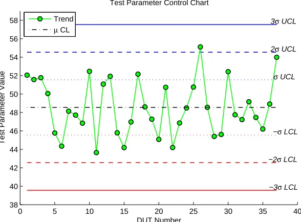
[image:37.612.174.468.67.284.2]

µ CL

Figure 2.3. Variable Control Chart. Test parameter trend showing µ

-centreline and σ-Upper Control Limit (UCL) and σ-Lower Control Limit

(LCL) levels. Only 1 DUT breaches the 2-σ UCL in this case.

fraction conforming charts and indices are used frequently in the calculation of First Pass Yield (FPY). FPY is simply the ratio of failures to total batch starts and is often quoted as percentage yield:

[1₋ F ailures

Entire batch]∗100

Monitoring FPY is a high level solution to a low level problem and is often used as an economic index to describe a process.

(38)

2.5. _{Multivariate Statistical Process Control} _{Literature Review}

2.5 Multivariate Statistical Process Control

Multivariate Statistical Process Control (MSPC) is simply a multivariate exten-sion of SPC. MSPC is increasingly recognised as a useful tool for providing an early warning of process changes, assignable plant faults, process disturbances and for giving the analyst a deeper understanding of the process. Computing technology, with improved data logging and analysis features, has increased the importance of multivariate analysis whereby the main objective is to identify the root causes of variation and take corrective action. Martin et al. (1999) use the term Multivariate Statistical Process Monitoring (MSPM) in place of MSPC, which conceptually gives a more appropriate description of the monitoring as-pect of process control strategies. Kourti et al. (1996) state that univariate SPC procedures are inadequate for most modern industrial processes, as they are tradi-tionally based on charting only a small number of final product quality variables. In Kourti (2002) the problem with monitoring a complex process through a uni-variate control strategy is illustrated. The author states that many industries made the transgression to MSPC a decade ago as monitoring a small number of variables (usually the final product quality variables) is totally inadequate and does not explain the underlying process fault conditions and emergence of ab-normal situations. Most industrial processes generate massive amounts of data on hundreds of process variables through various sensors arrays. The univariate SPC methodology of examining each variable singularly and independently makes the interpretation and diagnosis of a fault condition very difficult and convoluted MacGregor & Kourti (1995). This method only considers the magnitude of de-viation inherent in a single process variable independently of all other process variables. Simultaneous monitoring of individual variables separately will fail to recognise possible cross-correlations that may exist and will increase the insen-sitivity of the control charts for detection of out-of-control conditions, Samanta (2001). This can be quite misleading as not all the variables are independent and only a few underlying events are driving the process at any one time. The final product quality is defined by the simultaneous correct values of each variable, and therefore is a multivariate property. In summary, the product quality is a logical ‘AND’ of the test metrics.

(39)

2.5. _{Multivariate Statistical Process Control} _{Literature Review} variables for a particular process, fault conditions and abnormal situation can be detected more accurately.

Process monitoring is usually conducted at two levels, Marlin (2000). The first level is the immediate operation of the process by test operatives and technicians and the second is long term performance analysis by test engineers. Long term performance degradation is more difficult to diagnose than sudden process failure and is often dictated by the quality and quantity of historical data and any methods applied to extract relevant features.

When the data being analysed are large and correlated, the signal-to-noise ratio (SNR) is low in each variable. One of the main objectives in data compres-sion is to enhance the SNR, i.e. to minimise the noise terms which are assumed to be totally stochastic components.

2.5.1 Process Operation Data Characteristics

Data characteristics are vitally important in both process description and mod-elling. Wang (1999) lists the basics characteristics of process data where data volume, data dimension, uncertainty, noise, dynamic trends, sampling frequen-cies, data redundancy and complex interactions are important.

2.5.2 Classification of Batch Processes

(40)

2.5. _{Multivariate Statistical Process Control} _{Literature Review}

X2

X1 X2

X1

(a) (b)

Figure 2.4. Control ellipsoids. The elliptical regions represent in-control

data from separate batches, with the ‘_•’ points representing each mean and

the ‘

•

’ points represents the overall mean for (a)category 1 batch process

and (b)category 2 batch process.

with a significant separation between batch mean vectors. The observations are assumed to come from different multivariate normal distributions, Nd(µi,P), where µi, i = 1,2, ..., k, represents the population mean of the ith _{batch. The} difference among the batch means may be due to known of unknown causes. Figure 2.4 details each categorical condition. Figure 2.4 (a) shows in control production regions for batches taken from a Cat1 process containing two process variables,X1 andX2. The ellipsoids represent in control data from three separate

(41)

2.6. _{Unsupervised Learning Methods} _{Literature Review}

2.6 Unsupervised Learning Methods

The unsupervised learning methods of clustering and Principal Component Analy-sis (PCA) were used to analyse and reduce the dimensionality of the test data. These methods are discussed in Chapter 3.

2.6.1 Principal Component Analysis

Principal Component Analysis (PCA), is a key technique in the analysis of mul-tivariate data. It encompasses three possible objectives: description, interpreta-tion and modelling of the data, Krzanowski (2000). The methodology of PCA is reviewed in Section 3.2.2 and is comprehensively described in Jackson (1991) and Jolliffe (1986). Lane et al. (2001) develop a multi-group process represen-tation that overcomes the problem of having a single model for every product. In many industrial applications, the Principal Components (PCs) actually have physical interpretation and thus can be used as control variables in their own right. Jackson (1991) used PCA to examine audiometric data from a large num-ber of employees. The experimentation, while neither process or product related, made use of the data reduction feature inherent in PCA. PCA is used extensively within the Chemometrics field, Wold & Sj¨ostr¨om (1998), Ku et al. (1995) and Wise & Gallagher (1996), Semiconductor Etch and Monitoring Wise et al. (1999), Goodlin et al. (2002) and Skinner et al. (2002), Multivariate Statistical Process Control Kourti (2002), Wise et al. (1999), Lane et al. (2003), Simoglou et al. (2000), Exploratory data analysis in the food industry Pravdova et al. (2002) and Penza et al. (2001). Zuendorf (2003) detail the use of PCA in functional brain imaging in order to determine the patterns causing the greatest variance in the images. Asgharian & Hansson (2003) detail the use of PCA in determin-ing factors that are important in calculatdetermin-ing expected market returns and risk management of financial portfolios.

2.6.2 Monitoring Indices

(42)

2.7. _{Supervised Learning Methods} _{Literature Review} process monitoring then fault diagnosis should be performed to identify the cause (source) of the fault for corrective action. Process monitoring evaluates the op-erating condition of the process and assesses whether it is opop-erating within a predefined operating region, Leung (2002).

2.7 Supervised Learning Methods

In contrast to latent variable modelling, a supervised learning technique known as decision tree learning was employed with the same test data. The decision tree algorithm provides a tree capable of classifying test data with a high degree of accuracy. It is then tested with unseen data (i.e. data not used in the construction of the tree) for the purpose of fault classification and the performance evaluation. This is dependent on the induction method and cross-validation. A detailed description of decision trees and supervised classification is given in Chapter 4.1. In short, a decision tree is represented as a multi stage decision system in which the classes are sequentially rejected upon the arrival of a feature vector until the destination class (terminal node) is reached. A decision tree is constructed by recursively partitioning a learning sample of data in which the class label and the value of the predictor variables for each case is known

• Each internal node tests an attribute

• Each branch corresponds to an attribute value

• Each leaf node assigns a classification

2.7.1 Neural Networks

System representation, modelling and identification are fundamental to process engineering and other problem domains. It is often required to approximate a real system with an appropriate model given an input - output data set.

(43)

2.8. _{Chapter summary} _{Literature Review} NNs have been successfully applied to a number of real-world problems of large scale complexity. Their success can be attributed to their ability to offer a complex non-linear solution to a given problem not suitably accommodated by an algorithmic solution, Ritter et al. (1992).

Wong et al. (1997) survey and review journal articles on neural networks in business applications. The application base is diverse, but the largest problem domain is in production/process operation and the second largest is in finance.

NN’s have the to ability to present viable solutions to real-world problems, but in general form an appropriate part of a solution to a large scale problem. Noorossana et al. (2003) present a application of NNs to detection and classifica-tion of out-of-control signals.

Whilst supervised learning algorithms can perform well given adequate train-ing data, they have a number of drawbacks. Typically, they require a large training data set. This is of little importance in the data-rich environments of micro-electronics, batch process control and time series data but generation of a suitable training data set can be costly. Furthermore, in general it is not possible to incrementally add to the training data whilst training the classifier. If the training data is changed in any way then the entire training data set must be used to retrain the classifier.

2.8 Chapter summary

(44)

Chapter 3 Unsupervised Learning Methods

3.1 Exploratory Data Analysis

Statistical methods of analysis are only capable of ‘data modelling’ not ‘actual process modelling’ and this is an important realisation in any model develop-ment. Simply put, models are mathematical abstractions of a system which can vary greatly in complexity and usefulness. The primary goal is to capture the behaviour and to organise this information into a concise set of rules or metrics. In a multivariate framework, the structural complexity of a system is changed into a problem of high dimensionality. Abbott (1884) wrote of this very problem of dimensionality and visualisation in‘Flatland, A romance of many dimensions’. The ‘curse of dimensionality’ Bellman (1961) is the description of a problem that occurs when working with data in a high dimensional space. The complexity is exponential to the number of dimensions, which in statistical terms are the degrees of freedom. This dimensionality problem is illustrated in Figure 3.1 where Euclidean R3 _{space is defined by (}_x₁_{, x}₂_{, x}₃_{). Modelling a non-linear relationship}

through a set of input variables xi and output y can be achieved on the basis of

training data and partitioning the sample space. This however, is not an optimal solution. Firstly, the input variable is split into a number of intervals so that the value of a variable can be specified by indicating in which interval it lies. This leads to the division of the entire input space into a large number of cells (or blocks). Each of the training examples corresponds to a point in one of the cells and carries with it an associated value of the output variable y. Given a set of new input vectors xnew the corresponding output ynew could be determined by

finding which cell xnew falls in and returning the average for the the training

points in that cell. Increased precision requires the increase of the number of divisions along each axis.

(46)

X ₁

X ₂

X 3

Figure 3.1. d- dimensional Euclidean space Rd_. _{One method of mapping}

a d-dimensional space,(x1, x2, ..., xd), to an output variableyis to split the

space into a number of cells (or blocks) and specify a value ofy for each of

the cells. One major drawback of this method is the exponential growth of

the space with respect to d.

0 2

4 6

8 10

0 2 4 6 8 10

Z Dimension

3−Dimensional Space Mapping

X Dimension Y Dimension

Figure 3.2. Feature Space Mapping. Representing R3 _{space through a}

(10_×10_×10) feature map. Cells are shown for the x, y and z axes and

along the principal diagonal. For any (xi, yj, zk) triplet, an output y is

(47)

-1 0 1 2 3 4 5 6 7 8 9 10 -20

-10 0 10 20

x1 x2

-20 -10 0 10 20

(a) (b)

Figure 3.3. Methods of data representation in R2_{. (a)} _Cartesian _(b)

Parallel Coordinate Plot.

3.1.1 Parallel Coordinates Analysis

Parallel Coordinates Analysis (parallel-coords) was introduced by Inselberg (1981), in an attempt to rationalise high dimensional data structures. Parallel-coords is a two-dimensional technique for multidimensional data visualisation. It has proper-ties of low representational complexity, uniform treatment of all variables, works for any d-dimension and the display intuitively conveys information about the d-dimensional object it represents. Parallel-coords is an exploratory technique without any a priori bias. Any d-dimensional tuple (x1, x2, ..., xd) can be

vi-sualised as a polyline in parallel-coords, connecting the points x1, x2, ..., xd in d

parallel ordinates.

Figure 3.3 shows the representation of two vectors, x1 and x2, in both

carte-sian and parallel-coords. This is a trivial example, but it does convey the latter’s ability to extend beyond R2_{. Figure 3.3 (a) shows a cartesian or scatter plot of}

the two vectors. Figure 3.3 (b) shows two ordinates along the abscissa (x-axis) each displaying a vector. The transition from x1 → x2 is through a polyline and

each polyline passes through an axis at a location that indicates the observation’s value relative to all other values. Inselberg (1997) introduces the idea of parallel-coords as a space efficient method for representing large data sets and modelling relations between variables.

(48)

dimen-3.1. _{Exploratory Data Analysis} _{Unsupervised Learning Methods} sional space into correlated subsets that are more readily analysed.

3.1.2 Cluster Analysis

Cluster analysis is a pattern search method used in multivariate data structures and it can be applied to data that is quantitative (numerical), qualitative ( cate-gorical) or a mixture of both. The goal of clustering is to find an optimal grouping for which the variables within each cluster are similar but the clusters are dissimi-lar. This, in effect, has the tendency to find the natural groupings within the data which can be of significant benefit to the researcher or analyst. Clustering is a method where each data point is associated with its next closest point and likewise onwards until a specified amount of cluster centres are formed. There are many different clustering methods which attempt to identify and group similar data. It is necessary to have a measure of similarity or distance between the vectors in order to achieve this. Since distance increases as two points diverge, distance is actually a measure of ‘dissimilarity’, i.e. distance =similarity−₁

. Assuming a

Rd_{Euclidean space, the distance}_d_(x_,_{y) between two vectors}_x_{= (}_x₁_{, x}₂_{, ..., xn}₎T

and y = (y1, y2, ..., yn)T can be defined using one of the following distance

mea-sures

Euclidean = v u u t

n X

i=1

(xi−yi)2 (3.1a)

Manhattan = n X

i=1

|(xi−yi)| (3.1b)

Minkowski = " _n

X

i=1

(_|(xi−yi)|)p #1

p

(3.1c)

The Minkowski metric, Equation 3.1 c, becomes the Euclidean distance when p = 2 and the Manhattan or ‘city block’ distance when p = 1. The distance is called a metric if it satisfies to the following four axioms

• d(i, j)_≥0 (non-negative distance)

• d(i, j) = 0 (wheni=j)

(49)

3.1. _{Exploratory Data Analysis} _{Unsupervised Learning Methods} • d(i, j)_≤d(i, k) +d(k, j) (triangle inequality)

Another distance metric which accounts for the differing variances and co-variance amongst the variables in the data set is Mahalanobis distance and it is defined as

Mahalanobis = r

(xi−yi)T X−1

(xi−yi) (3.2)

where Pis the covariance matrix.

Tryon & Bailey (1970) outline the concept of cluster analysis which was first introduced by Tryon in 1939 although an earlier reference to clustering and the concept of measuring likeness was given by Karl Pearson in his 1926 paper ”On the Coefficient of Radical Likeness”.

Clustering techniques and algorithms are well documented in literature. Bha-tia & Deogun (1998) and Carpineto & Romano (1996) describe information re-trieval and document classification using conceptual clustering techniques. Judd et al. (1998) use clustering in data mining and image analysis. Hartigan (1984) describes data clustering and unsupervised learning in multidimensional data. An indepth and thorough review of clustering is given in Kain et al. (1999). The termclustering is used widely in different research communities to describe meth-ods of grouping unlabelled data. Humans perform competitively with automatic clustering procedures in two dimensions, but most real problems involve cluster-ing in higher dimensions, Kain et al. (1999). Successful clustercluster-ing is achieved when there is high within class similarity (homogeneity) and low between class similarity (heterogeneity) between the cluster groups. Clustering also has the ability to discover some hidden patterns in the data and organise large amounts of data both quickly and efficiently. Clustering performance is dependent upon the distance metric and its implementation.

(50)

3.1.3 Hierarchical Clustering

Hierarchical methods work by grouping the data into a tree of clusters using a computationally efficient technique. When the dimension of the data set is large, it is generally not feasible to examine all possible clustering possibilities. The number of ways of partitioning a set of n items into g clusters is given by

N(n, g) = 1 g!

g X

k=1

g k

(₋1)g−k_kn _(3.3)

in Seber (1984). This can be further approximated by

N(n, g)≅ g

n g!

which is large even for moderate values of n and g. For example, the number of ways of partitioning 20 items into 10 groups, N(20,10) from Equation 3.3 is

≅ ₂_.₇₆_×₁₀13_{. Hierarchical methods therefore permit the analyst to search for}

reasonable solutions without having to look at all the possible clustering arrange-ments. This grouping can be either agglomerative or divisive. Agglomerative clustering methods is a bottom-up approach and starts with each object forming a separate cluster. This cluster successively merges the items (or groups of items) until a stopping criterion is reached. Divisive clustering is a top-down approach and starts with all items clustered together. This cluster is iteratively split into smaller clusters until a stopping criterion is reached. Of the two, agglomerative methods are more commonly used.

Agglomerative Clustering

One of the most commonly used agglomerative clustering methods is simple link-age, more commonly known as Nearest Neighbour clustering. In essence, this is the minimum distance between a point yi in cluster A and a point yj in cluster B and is defined as

D(A, B) =min_{d(y1, yj), foryi in A andyj in B} (3.4)

where d(y1, yj) is a distance metric such as the Euclidean distance in

(51)

3.1. _{Exploratory Data Analysis} _{Unsupervised Learning Methods} smallest distance are merged. This is an iterative process and the final result is achieved when the pair with the minimal distance is merged into a single clus-ter. It is perhaps useful to visualise the concept of nearest neighbour clustering with an example. Figure 3.4 (a) shows a Voronoi diagram on a two class data set_−→{

•

,⋆_}_{. This is a simplified classification problem given a new vector}

(query point q) to classify. A voronoi diagram is constructed by partitioning a plane with n points into convex polygons such that each polygon contains ex-actly one generating point and every point in each given polygon is closer to its generating point than to any other. Query points outside the convex polygons are closer to some other training example. In Figure 3.4 (a), the 1-NN algorithm classifies q as ‘⋆_{’ whereas in Figure 3.4 (b) the 7-NN algorithm classifies} q as ‘

•

’ from a majority count in the decision region. This region is depicted by ‘

’. Mitchell (1997) states that the hypothesis spaceH is not implicity considered by thek-NN algorithm, but rather, the algorithm computes the classification of each new query point or instance as needed. The data set used to construct the voronoi diagram can be represented through a connection dendrogram. As clustering is an unsupervised learning technique, the data are without any class labels. This is shown in Figure 3.5, where each sample is treated as a singleton cluster at the onset of the analysis and subsequently pooled with its nearest neighbour to form a new cluster, Cnew. The colouring of lines in the dendrogram in Figures 3.5 (a) and (b) is to illustrate the clustering effect inherent in the data. Figure 3.5 (a) shows two main cluster groups, indicated by theblueand redlines. The vertical lines indicate which samples are linked and the horizontal lines indicate the length of a link, i.e. the distance between the linked groups. Of interest to note is that data points 11 & 13 have the smallest distance metric (i.e. they are the closest together) and points 12 & 14 are somewhat removed from both cluster centres. Figure 3.5 (b) shows the result from the k-means algorithm. It can be seen that there is a slight difference in cluster assignments between the points (shown by

the green lines). Clustering techniques are widely used for pattern recognition

(52)

0 0.2 0.4 0.6 0.8 1

0 0.1 0.2 0.3 0.4 0.5 0.6 0.7 0.8 0.9 1

Voronoi Diagram

query point, q

(a)

0 0.2 0.4 0.6 0.8 1

0 0.1 0.2 0.3 0.4 0.5 0.6 0.7 0.8 0.9 1

Voronoi Diagram

query point, q

(b)

Figure 3.4. Voronoi Tesselation in R2 _{showing Query Point,} _q_with

Near-est Neighbours (NN). (a) 1-NN classifies q as ⋆ (b) 7-NN classifies q as

(53)

3.2. _{Dimension Reduction Methods} _{Unsupervised Learning Methods}

0 0.05 0.1 0.15 0.2 0.25 0.3 0.35 0.4 Distance to k−NN

1 2 3 4 5 6 7 8 9 10 11 12 13 14 15 Dendrogram

0 0.1 0.2 0.3 0.4 0.5 0.6 Distance to K−Means Nearest Group 1 2 3 4 5 6 7 8 9 10 11 12 13 14 15 Dendrogram (a) (b)

Figure 3.5. Cluster Dendrogram. (a) A connection dendrogram

con-structed using the k-NN algorithm and (b) The k-means algorithm, using

the same data set as Figure 3.4. The ‘_|’ lines indicate which samples are

linked together, and the ‘ —’ lines indicate the length of the link (i.e. the distance between two linked groups).

3.1.4 Non-Hierarchical Clustering

A common non-hierarchical method is k-means clustering. This method allows items to be moved from one cluster to another, a reallocation not applicable in hierarchical clustering. Initially, k items are chosen as seeds and data is assigned to the cluster with the nearest seed based on a distance metric (Euclidean). When the cluster has more than one member, the cluster seed is replaced by the centroid. This procedure is sensitive to the initial seed choice, but can be an improvement in clustering performance due to the reallocation of points. Clustering techniques can be problematical for very high dimensional data and time series data as many clustering algorithms are computationally expensive.

3.2 Dimension Reduction Methods

(54)

com-3.2. _{Dimension Reduction Methods} _{Unsupervised Learning Methods} ponents, monitor fewer process variables, uncorrelate data and assess process performance. Perhaps the most widely used technique is Principal Component Analysis.

3.2.1 Multivariate Data Modelling

Choosing the correct procedure to successfully represent and model multivariate data structures is a difficult task. Martens & Martens (2001) define Bi-Linear Modelling (BLM) as a multivariate method of information extraction which is dependent upon both the data type and modelling algorithm. BLM is built on a combination of multivariate analysis and statistical regression theory, where a methodology is used to extract relevant information from input data and com-bined with cross-validation and graphical analysis. Models can be used to give a concise and simplified representation of an otherwise complex system (or process) and these allow for quantitative interpretation and prediction. There is a trade off between model complexity and cognisance, therefore a trade-off between the two is important.

The methods used in modelling data are multi-disciplinarian as they can be analogously used in Chemometrics, Econometrics, Psychology, Biology, Statis-tics, Mathematics and Engineering. The factors that are different between these disciplines are data structures (i.e. numerical, continuous, discrete, categorical or mixed mode) and the required ‘input-output’ relationships. There are other fac-tors that are very significant to the outcome such as philosophical and technical issues that also need consideration.

3.2.2 Principal Component Analysis

Principal Component Analysis (PCA) is derived from the hypothesis that data variance carries with it information. This is an underlying assumption of PCA. The basic methodology of PCA is used in many different disciplines, each with their own definitions and conventions. In statistics it is known as PCA, in nu-merical analysis as Singular Value Decomposition (SVD) or Eigenanalysis and in Pattern Classification and Signal Processing as Karhunen-Lo´eve transform.

(55)

3.2. _{Dimension Reduction Methods} _{Unsupervised Learning Methods} multivariate techniques which has found wide spread application in a variety of substantive areas, Krzanowski (2002). PCA was first introduced by Pearson (1901) in his paper entitled “On lines and planes of closest fit to systems of points in space”, The London, Edinburgh and Dublin Philosophical Magazine and Journal of Science. Pearson, through a geometrical viewpoint, introduced the concept of ‘line of best fit’ and the ‘line of worst fit’ through the data, subsequently known asPrincipal Components. Some thirty years later, Hotelling (1933) independently made reference to principal components, and in contrast, took an algebraic approach that established Pearson’s principal components were also the orthogonal directions in space that successively maximised the variance of the data. Therefore it holds that the d-dimensional subspace of closest fit to the data is also the subspace in which the variance is maximised. Much has been built on the earlier contributions to PCA and Anderson (1963) developed the distributional theory underlying PCA from a statistical perspective.

PCA is concerned with explaining the variance-covariance structure of a data set through a reduced set oflinear combinations of the original variables. In short, the objective of PCA is to represent a variable in terms of several underlying factors. Succinctly, PCA can perform:

Data Reduction Although the original data set may contain p variables, it is often the case that much of the variability can be accounted for by a smaller number (m) of principal components.

Data Interpretation Relationships that were previously unsuspected can com-monly be identified through PCA.

In Montgomery (2001), PCA is referred to as a Latent Structures Modelling technique because of the analogy with photographic film where a hidden or latent image resides as a result of light interacting with the chemical surface of the film. PCA is similar in nature Factor Analysis and these two techniques‘look inside’ a set of variables and attempt to assess the structure of the data. The most simple theoretical model for describing a variable in terms of several other variables is a linear one thus, PCA linearly transforms an original set of variables X = [X1, X2, ..., Xp]T into a substantially smaller set of uncorrelated variables Z. The

Multivariate statistical methods for fault detection and classification