Improving Language Modeling using Densely Connected Recurrent Neural Networks

Improving Language Modeling using

Densely Connected Recurrent Neural Networks

Fr´ederic Godin, Joni Dambre and Wesley De Neve

IDLab - ELIS, Ghent University - imec, Ghent, Belgium firstname.lastname@ugent.be

Abstract

In this paper, we introduce the novel con-cept of densely connected layers into re-current neural networks. We evaluate our proposed architecture on the Penn Treebank language modeling task. We show that we can obtain similar perplex-ity scores with six times fewer parame-ters compared to a standard stacked 2-layer LSTM model trained with dropout (Zaremba et al., 2014). In contrast with the current usage of skip connections, we show that densely connecting only a few stacked layers with skip connections al-ready yields significant perplexity reduc-tions.

1 Introduction

Language modeling is a key task in Natural Lan-guage Processing (NLP), lying at the root of many NLP applications such as syntactic parsing (Ling et al.,2015), machine translation (Sutskever et al., 2014) and speech processing (Irie et al.,2016).

In Mikolov et al. (2010), recurrent neural net-works were first introduced for language model-ing. Since then, a number of improvements have been proposed. Zaremba et al. (2014) used a stack of Long Short-Term Memory (LSTM) lay-ers trained with dropout applied on the outputs of every layer, whileGal and Ghahramani(2016) and Inan et al. (2017) further improved the per-plexity score using variational dropout. Other im-provements are more specific to language model-ing, such as adding an extra memory component (Merity et al., 2017) or tying the input and out-put embeddings (Inan et al.,2017;Press and Wolf, 2016).

To be able to train larger stacks of LSTM lay-ers, typically four layers or more (Wu et al.,2016),

skip or residual connections are needed.Wu et al. (2016) used residual connections to train a ma-chine translation model with eight LSTM layers, whileVan Den Oord et al.(2016) used both resid-ual and skip connections to train a pixel recurrent neural network with twelve LSTM layers. In both cases, a limited amount of skip/residual connec-tions was introduced to improve gradient flow.

In contrast, Huang et al. (2017) showed that densely connecting more than 50 convolutional layers substantially improves the image classifica-tion accuracy over regular convoluclassifica-tional and resid-ual neural networks. More specifically, they intro-duced skip connections between every input and

everyoutput ofeverylayer.

Hence, this motivates us to densely connect all layers within a stacked LSTM model using skip connections between every pair of layers.

In this paper, we investigate the usage of skip connections when stacking multiple LSTM layers in the context of language modeling. When every input of every layer is connected with every output of every other layer, we get a densely connected recurrent neural network. In contrast with the cur-rent usage of skip connections, we demonstrate that skip connections significantly improve perfor-mance when stacking only afewlayers. Moreover, we show that densely connected LSTMs need fewer parameters than stacked LSTMs to achieve similar perplexity scores in language modeling.

2 Background: Language Modeling A language model is a function, or an algo-rithm for learning such a function, that captures the salient statistical characteristics of sequences of words in a natural language. It typically al-lows one to make probabilistic predictions of the next word, given preceding words (Bengio,2008). Hence, given a sequence of words[w1, ...wT], the

goal is to estimate the following joint probability:

P r(w1, ..., wT) = T

∏

t=1

P r(wt|wt−1, ..w1) (1)

In practice, we try to minimize the negative log-likelihood of a sequence of words:

Lneg(θ) =− T

∑

t=1

log(P r(wt|wt−1, ..w1)). (2)

Finally, perplexity is used to evaluate the perfor-mance of the model:

P erplexity = exp

(_L

neg(θ)

T )

(3)

3 Methodology

Language Models (LM) in which a Recur-rent Neural Network (RNN) is used are called Recurrent Neural Network Language Models (RNNLMs) (Mikolov et al.,2010). Although there are many types of RNNs, the recurrent step can formally be written as:

ht =f_θ(xt,ht−1) (4)

in which xt andht are the input and the hidden state at time step t, respectively. The functionfθ

can be a basic recurrent cell, a Gated Recurrent Unit (GRU), a Long Short Term Memory (LSTM) cell, or a variant thereof.

The final predictionP r(wt|wt−1, ..w1)is done

using a simple fully connected layer with a soft-max activation function:

yt =softmax(W ht+b). (5)

Stacking multiple RNN layers To improve per-formance, it is common to stack multiple recurrent layers. To that end, the hidden state of a a layerl is used as an input for the next layerl+ 1. Hence, the hidden statehl,tat time steptof layerlis cal-culated as:

xl,t=hl−1,t, (6)

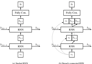
hl,t=fθl(xl,t,hl,t−1). (7) An example of a two-layer stacked recurrent neu-ral network is illustrated in Figure1a.

However, stacking too many layers obstructs fluent backpropagation. Therefore, skip connec-tions or residual connecconnec-tions are often added. The latter is in most cases a way to avoid increasing the

size of the input of a certain layer (i.e., the inputs are summed instead of concatenated).

A skip connection can be defined as:

xl,t = [hl−1,t;hl−2,t] (8)

while a residual connection is defined as:

xl,t=hl−1,t+hl−2,t. (9)

Here, xl,t is the input to the current layer as de-fined in Equation7.

Densely connecting multiple RNN layers In analogy with DenseNets (Huang et al., 2017), a densely connected set of layers has skip connec-tions from every layer to every other layer. Hence, the input to RNN layerlcontains the hidden states of all lower layers at the same time stept, includ-ing the output of the embeddinclud-ing layeret:

xl,t= [hl−1,t;...;h1,t;et]. (10)

Due to the limited number of RNN layers, there is no need for compression layers, as introduced for convolutional neural networks (Huang et al., 2017). Moreover, allowing the final classification layer to have direct access to the embedding layer showed to be an important advantage. Hence, the final classification layer is defined as:

yt=softmax(W[hL,t;...;h1,t;et] +b). (11)

An example of a two-layer densely connected re-current neural network is illustrated in Figure1b.

4 Experimental Setup

We evaluate our proposed architecture on the Penn Treebank (PTB) corpus. We adopt the standard train, validation and test splits as described in Mikolov and Zweig(2012), containing 930k train-ing, 74k validation, and 82k test words. The vocabulary is limited to 10,000 words. Out-of-vocabulary words are replaced with an UNK to-ken.

RNN

h1,t

RNN

et

h2,t

h2,t

h2,t−1

h1,t−1 h1,t

yt

Fully Con.

(a) Stacked RNN

RNN

h1,t

RNN

et

h2,t

h2,t

h2,t−1

h1,t−1 h1,t

yt

Fully Con.

et

h1,t

et

RNN

RNN

(b) Densely connected RNN

Figure 1: Example architecture for a model with two recurrent layers.

LSTM layers, we also evaluate a model with three stacked LSTM layers, and experiment with two, three, four and five densely connected LSTM lay-ers. The hidden state size of the densely connected LSTM layers is either 200 or 650. The size of the embedding layer is always 200.

We applied standard dropout on the output of every layer. We used a dropout probability of 0.6 for models with size 200 and 0.75 for mod-els with hidden state size 650 to avoid overfitting. Additionally, we also experimented with Varia-tional Dropout (VD) as implemented inInan et al. (2017). We initialized all our weights uniformly in the interval [-0.05;0.05]. In addition, we used a batch size of 20 and a sequence length of 35 dur-ing traindur-ing. We trained the weights usdur-ing stan-dard Stochastic Gradient Descent (SGD) with the following learning rate scheme: training for six epochs with a learning rate of one and then ap-plying a decay factor of 0.95 every epoch. We constrained the norm of the gradient to three. We trained for 100 epochs and used early stopping. The evaluation metric reported is perplexity as de-fined in Equation3. The number of parameters re-ported is calculated as the sum of the total amount of weights that reside in every layer.

Note that apart from the exact values of some hyperparameters, the experimental setup is identi-cal toZaremba et al.(2014).

5 Discussion

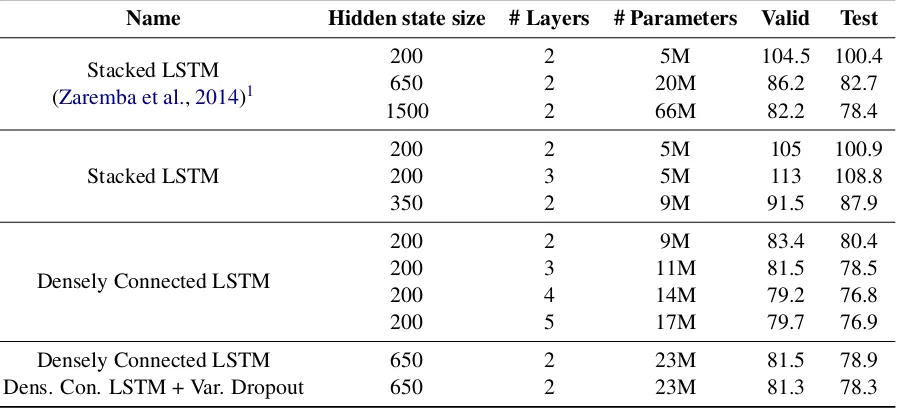
The results of our experiments are depicted in Ta-ble1. The first three results, marked withstacked LSTM (Zaremba et al.,2014), follow the setup of Zaremba et al. (2014) while the other results are obtained following the setup described in the pre-vious section.

The smallest densely connected model which only uses two LSTM layers and a hidden state size of 200, already reduces the perplexity with 20% compared to a two-layer stacked LSTM model with a hidden state size of 200. Moreover, in-creasing the hidden state size to 350 to match the amount of parameters the two-layer densely con-nected LSTM model contains, does not result in a similar perplexity. The small densely connected model still realizes a 9% perplexity reduction with an equal amount of parameters.

Table 1: Evaluation of densely connected recurrent neural networks for the PTB language modeling task.

Name Hidden state size # Layers # Parameters Valid Test

Stacked LSTM (Zaremba et al.,2014)1

200 2 5M 104.5 100.4

650 2 20M 86.2 82.7

1500 2 66M 82.2 78.4

Stacked LSTM 200200 23 5M5M 105113 100.9108.8

350 2 9M 91.5 87.9

Densely Connected LSTM

200 2 9M 83.4 80.4

200 3 11M 81.5 78.5

200 4 14M 79.2 76.8

200 5 17M 79.7 76.9

Densely Connected LSTM 650 2 23M 81.5 78.9

Dens. Con. LSTM + Var. Dropout 650 2 23M 81.3 78.3

Increasing the hidden state size is less beneficial compared to adding an additional layer, in terms of parameters used. Moreover, a dropout probabil-ity of 0.75 was needed to reach similar perplexprobabil-ity scores. Using variational dropout with a probabil-ity of 0.5 allowed us to slightly improve the per-plexity score, but did not yield significantly better perplexity scores, as it does in the case of stacked LSTMs (Inan et al.,2017).

In general, adding more parameters by in-creasing the hidden state and performing subse-quent regularization, did not improve the perplex-ity score. While regularization techniques such as variational dropout help improving the infor-mation flow through the layers, densely connected models solve this by adding skip connections. In-deed, the higher LSTM layers and the final classi-fication layer all have direct access to the current input word and corresponding embedding. When simply stacking layers, this embedding informa-tion needs to flow through all stacked layers. This poses the risk that embedding information will get lost. Increasing the hidden state size of every layer improves information flow. By densely connect-ing all layers, this issue is mitigated. Outputs of lower layers are directly connected with higher layers, effectuating efficient information flow.

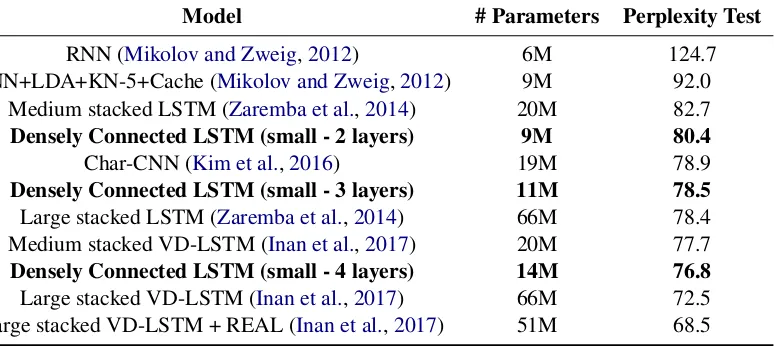
Comparison to other models In Table2, we list a number of closely related models. A densely 1_{There are no results reported inZaremba et al.(2014)} for a small network with dropout. These are our own results, following the exact same setup as for the medium-sized ar-chitecture.

connected LSTM model with an equal number of parameters outperforms a combination of RNN, LDA and Kneser Ney (Mikolov and Zweig,2012). Applying Variational Dropout (VD) (Inan et al., 2017) instead of regular dropout (Zaremba et al., 2014) can further reduce the perplexity score of stacked LSTMs, but does not yield satisfactory re-sults for our densely connected LSTMs. How-ever, a densely connected LSTM with four lay-ers still outperforms a medium-sized VD-LSTM while using fewer parameters. Inan et al. (2017) also tie the input and output embedding together (cf. model VD-LSTM+REAL). This is, however, not possible in densely connected recurrent neural networks, given that the input and output embed-ding layer have different sizes.

6 Conclusions

Table 2: Comparison to other language models evaluated on the PTB corpus.

Model # Parameters Perplexity Test

RNN (Mikolov and Zweig,2012) 6M 124.7 RNN+LDA+KN-5+Cache (Mikolov and Zweig,2012) 9M 92.0

Medium stacked LSTM (Zaremba et al.,2014) 20M 82.7

Densely Connected LSTM (small - 2 layers) 9M 80.4

Char-CNN (Kim et al.,2016) 19M 78.9

Densely Connected LSTM (small - 3 layers) 11M 78.5

Large stacked LSTM (Zaremba et al.,2014) 66M 78.4 Medium stacked VD-LSTM (Inan et al.,2017) 20M 77.7

Densely Connected LSTM (small - 4 layers) 14M 76.8

Large stacked VD-LSTM (Inan et al.,2017) 66M 72.5 Large stacked VD-LSTM + REAL (Inan et al.,2017) 51M 68.5

Acknowledgments

The research activities as described in this pa-per were funded by Ghent University, imec, Flan-ders Innovation & Entrepreneurship (VLAIO), the Fund for Scientific Research-Flanders (FWO-Flanders), and the EU.

References

Yoshua Bengio. 2008. Neural net language models.

Scholarpedia3(1):3881. revision #91566.

Yarin Gal and Zoubin Ghahramani. 2016. A theoret-ically grounded application of dropout in recurrent neural networks. InAdvances in Neural Information Processing Systems.

Gao Huang, Zhuang Liu, Kilian Q Weinberger, and Laurens van der Maaten. 2017. Densely connected convolutional networks. InProceedings of the IEEE Conference on Computer Vision and Pattern Recog-nition.

Hakan Inan, Khashayar Khosravi, and Richard Socher. 2017. Tying word vectors and word classifiers: A loss framework for language modeling. In Proceed-ings of the International Conference on Learning Representations.

Kazuki Irie, Zolt´an T¨uske, Tamer Alkhouli, Ralf Schl¨uter, and Hermann Ney. 2016. Lstm, gru, high-way and a bit of attention: an empirical overview for language modeling in speech recognition. In Pro-ceedings of Interspeech.

Yoon Kim, Yacine Jernite, David Sontag, and Alexan-der M. Rush. 2016. Character-aware neural lan-guage models. InProceedings of the Thirtieth AAAI Conference on Artificial Intelligence.

Wang Ling, Chris Dyer, Alan W. Black, Isabel Tran-coso, Ramon Fermandez, Silvio Amir, Lus Marujo,

and Tiago Lus. 2015. Finding function in form: Compositional character models for open vocabu-lary word representation. In Proceedings of the International Conference on Empirical Methods in

Natural Language Processing.

Stephen Merity, Caiming Xiong, James Bradbury, and Richard Socher. 2017. Pointer sentinel mixture models. InProceedings of the International Con-ference on Learning Representations.

Tomas Mikolov, Martin Karafit, Luks Burget, Jan Cer-nock, and Sanjeev Khudanpur. 2010. Recurrent neu-ral network based language model. InProceedings of Interspeech.

Tomas Mikolov and Geoffrey Zweig. 2012. Context dependent recurrent neural network language model.

In Proceedings of the IEEE Workshop on Spoken

Language Technology.

Ofir Press and Lior Wolf. 2016. Using the output embedding to improve language models. CoRR

abs/1608.05859.http://arxiv.org/abs/1608.05859. Ilya Sutskever, Oriol Vinyals, and Quoc V. Le. 2014.

Sequence to sequence learning with neural net-works. InProceedings of the International Confer-ence on Neural Information Processing Systems. A¨aron Van Den Oord, Nal Kalchbrenner, and Koray

Kavukcuoglu. 2016. Pixel recurrent neural net-works. In Proceedings of the 33rd International Conference on International Conference on Ma-chine Learning.

Yonghui Wu, Mike Schuster, and Zhifeng Chen et al. 2016. Google’s neural machine transla-tion system: Bridging the gap between human and machine translation. CoRR abs/1609.08144. http://arxiv.org/abs/1609.08144.