Proceedings of the SIGDial 2019 Conference, pages 46–55 46
Simple, Fast, Accurate Intent Classification and Slot Labeling for
Goal-Oriented Dialogue Systems
Arshit Gupta∗
Amazon AI Seattle
John Hewitt∗†
Stanford University Palo Alto
Katrin Kirchhoff
Amazon AI Seattle
Abstract
With the advent of conversational assistants like Amazon Alexa, Google Now, etc., dia-logue systems are gaining a lot of traction, especially in industrial settings. These sys-tems typically include a Spoken Language un-derstanding component which consists of two tasks: Intent Classification (IC) and Slot La-beling (SL). Generally, these two tasks are modeled together jointly to achieve best per-formance. However, this joint modeling adds to model obfuscation. In this work, we first design framework for a modularization of joint IC-SL task to enhance architecture trans-parency. Then, we explore a number of self-attention, convolutional, and recurrent models, contributing a large-scale analysis of model-ing paradigms for IC+SL across two datasets. Finally, using this framework, we propose a class of ‘label-recurrent’ models that are non-recurrent apart from a 10-dimensional repre-sentation of the label history, and show that our proposed systems are highly accurate (achiev-ing over 30% error reduction in SL over the state-of-the-art on the Snips dataset), as well as fast, at 2x the inference and 2/3 to 1/2 the train-ing time of comparable recurrent models, thus giving an edge in critical real-world systems.
1 Introduction
At the core of task-oriented dialogue systems are spoken language understanding (SLU) models, tasked with determining the intent of users’ ut-terances and labeling semantically relevant words at each turn of the conversation. Performance on these tasks, known as intent classification (IC) and slot labeling (SL), upper-bounds the utility of such dialogue systems. A large body of recent research has improved these models through the use of re-current neural networks, encoder-decoder archi-tectures, and attention mechanisms. However, for
∗
Equal Contribution
†
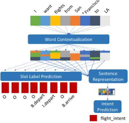
[image:1.595.313.520.226.424.2]Work performed while at Amazon AI
Figure 1:A general framework of joint IC+SL, decoupling modeling tasks to permit the analysis of each component in-dependently.
production dialogue systems in particular, system speed is at a premium, both during training and in real-time inference.
In this work, we propose fully non-recurrent and label-recurrent model paradigms including self-attention and convolution for comparison to state-of-the-art recurrent models in terms of ac-curacy and speed. To achieve this, we design a framework for joint IC-SL models that is modu-larized into different components and makes the task agnostic to type of neural network used. This, in turn, makes the model architecture simpler, easy to understand and renders the task network agnos-tic, allowing for easier plug and play using existing components, such as pre-trained contextual word embeddings (Devlin et al., 2019), etc. This is es-sential for easier model debugging and quicker ex-perimentation, especially in industrial settings.
label-recurrent, and non-recurrent. Recent state-of-the-art models fall into the first category, as encoder-decoder architectures have recurrent en-coders to perform word context encoding, and pre-dict slot label sequences using recurrent decoders that use both word and label information as they decode (Hakkani-T¨ur et al.,2016;Liu and Lane,
2016; Li et al., 2018). In second category, we have ‘non-recurrent’ networks: fully feed-forward, attention-based, or convolutional models, for ex-ample. Lastly, we have a class of label-recurrent models, inspired by structured sequential mod-els like conditional random fields on top of non-recurrent word contextualization components. In this class of models, slot label decoding proceeds such that label sequences are encoded by a recur-rent component, but word sequences are not.
Our contributions are:
• A class of label-recurrent convolutional mod-els that achieve state-of-the-art performance on Snips and competitive performance on ATIS while maintaining faster training and inference speeds than fully-recurrent models
• A new modular framework for joint IC-SL models that permits the analysis of individ-ual modeling components that decomposes these joint models into separate components forword context encoding,summarization of the sentence into a single vector for intent classification, andmodeling of dependencies in the output spaceof slot label sequences.
• In-depth analysis of different word contextu-alizations for Spoken Language Understand-ing task (for instance, providUnderstand-ing evidence for the intuition that explicitly focusing on lo-cal context is a useful architectural inductive prior for slot labeling)
2 Prior Work
There is a large body of research in applying recur-rent modeling advances to intent classification and slot labeling (frequently called spoken language understanding). Traditionally, for intent classifica-tion, word n-grams were used with SVM classifier (Haffner et al.,2003) and Adaboost (Schapire and Singer,2000). For the SL task, CRFs (Gorin et al.,
1997) have been used in the past.
Recently, a larger focus has been on joint mod-eling of IC and SL tasks. Long short-term mem-ory recurrent neural networks (Hochreiter and
Schmidhuber, 1997) and Gated Recurrent Unit models (Cho et al.) were proposed for slot labeling byYao et al.(2014) andZhang and Wang(2016) respectively, while Guo et al.(2014) used recur-sive neural networks. Subsequent improvements to recurrent neural modeling techniques, like bidi-rectionality and attention (Bahdanau et al.,2014) were incorporated into IC+SL in recent years as well (Hakkani-T¨ur et al., 2016; Liu and Lane,
2016).Li et al. (2018) introduced a self-attention based joint model where they used self-attention and LSTM layers along with the gating mecha-nism for this task.
Non-recurrent modeling for language has been re-visited recently, even as recurrent techniques continue to be dominant. Dilated CNNs (Yu and Koltun,2015) with CRF label modeling were ap-plied to named entity recognition byStrubell et al.
(2017), and earlier were applied to SL by Xu and Sarikaya(2013). Convolutional and attention-based sentence encoders have been applied in complex tasks, including machine translation, nat-ural language inference, and parsing. (Gehring et al., 2017; Vaswani et al., 2017; Shen et al.,
2017;Kitaev and Klein,2018) We draw from both of these bodies of work to propose a simple yet highly effective family of IC+SL models.
3 A general framework of joint IC+SL
Intent classification and slot labeling take as input an utterance x1:T = {x1,x2, ...xT}, composed
of wordsxi and of lengthT. Models construct a
distribution over intents and slot label sequences given the utterance. One intent is assigned per ut-terance and one slot label is assigned per word:
P(l1:T, c|x1:T) (1)
where c ∈ I, a fixed set of intents, and li ∈ L,
a fixed set of slot labels. Models are trained to minimize the cross-entropy loss between the as-signed distribution and the training data. To the end of constructing this distribution, our frame-work explicitly separates the following compo-nents, which are explicitly or implicitly present in all joint IC+SL systems (Figure1):
3.1 Word contextualization
In this component, word representations are en-riched with sentential context. Each word xi is
assigned a contextualized representation hi. To
ease layering these components, we keep the di-mensionality the same as the word embeddings;
hi ∈ Rdx. Our study consists mainly of vary-ing this component across models, which are de-scribed in detail in Section 4. In all models, we assume independence of intent classification and slot labeling given the learned representations:
P(l1:T, c|h1:T) =P(l1:T|h1:T)P(c|h1:T) (2)
3.2 Sentence representation
In this component, the output of the word contex-tualization component is summarized in a single vector,
s=SentenceRepr(h1:T) (3)
wheres ∈ Rdx. For all our experiments, we keep this component constant, using a simple attention-like pooling which is the weighted sum of word contextualization for each position in the sentence. These weights are computed using softmax over these individual word contextualizations
While simple, this model permits word con-textualization components freedom in how they encode sentential information; for example, self-attention models may spread full-sentence infor-mation across all words, whereas 1-directional LSTMs may focus full-sentence information in the last word’s vector.
3.3 Intent prediction
In this component, the sentence representation is used as features to predict the intent of the utter-ance. For all experiments, we keep this compo-nent fixed as well, using a simple two-layer feed-forward block on top ofs.
3.4 Slot label prediction
In this component, the output of the word contex-tualization component is used to construct a distri-bution over slot label sequences for the utterance. We decompose the joint probability of the label sequence given the contextualized word represen-tations into a left-to-right labeling:
P(l1:T|h1:T) = T Y
i=1
P(li|h1:T, l1:i−1) (4)
In our experiments, we explore two models for slot prediction, one fully-parallelizable because of strong independence assumptions, the other per-mitting a constrained dependence between label-ing decisions that we call ‘label-recurrent’.
Independent slot prediction The first is a non-recurrent model, which assumes indepdencence between all labeling decisions once given h1:T,
as well as independence from all word represen-tations except that of the word being labeled:
P(li|h1:T, l1:i−1) =P(li|hi) (5)
This model is fully parallelizable on GPU archi-tectures, and the probability of each labeling deci-sion is modeled according to
P(li|h1:T) =softmax(W(3)pi,SL+b(3)) (6)
pi,SL =tanh(W(4)hi+b(4)) (7)
hence, SL prediction features are learned using each contextualized word independently.
Label-recurrent slot prediction The second class of slot prediction models we consider lead to our classification, ‘label-recurrent.’1 These mod-els permit dependence of labeling decisions on the sequence of decisions made so far, but keep the independence assumption on the word representa-tions:
P(li|h1:T, l1:i−1) =P(li|l1:i−1,hi) (8)
Notably, this family of models excludes traditional encoder-decoder models, since the decoder com-ponent uses labeling decisions l1:i−1 and earlier
word representations h1:i−1 to influence the
pre-dictor featurespi,SL. However, it includes models
such as CNN-CRF.
The space of label sequences in slot labeling is much smaller than the space of word sequences. This adds minimal computational burden and per-mits the model to benefit from GPU parallelism duringh1:T computation.
For our experiments, we propose a single label-recurrent model, which encodes labeling histories l1:−i using only a 10-dimensional LSTM. First,
slot labels are embedded, such that for eachl∈ L, we havel∈ Rdl. An initial tag history state,htag
0 ,
is randomly initialized. Each tag decision is fed
1We use this term for clarity in language, not to claim that
along with the previous tag history state to the LSTM, which returns the next tag history state:
htagi =LSTM(li−1,htagi−1). (9)
We omit a precise description of the LSTM model here for space, referring the reader to (Hochreiter and Schmidhuber,1997).
The tag history is used at each prediction step as additional inputs to construct the predictor fea-turespi,SL, replacing Eqn.7with:
pi,SL=tanh(W(5)[hi;htagi ] +b(5)) (10)
where [a;b] denotes concatenation. This model and other label-recurrent models are not only par-allelizable more than fully-recurrent models, but also provide an architectural inductive bias, sepa-rating modeling of tag sequences from modeling of word sequences. In our experiments, we per-form greedy decoding to maintain a high decoding speed.
4 Word contextualization models
In this section, we describe word contextualization models with the goal of identifying non-recurrent architectures that achieve high accuracy and faster speed than recurrent models.
4.1 Feed-forward model
In this model, we seth1:T = x1:T +a1:T, where a1:T is a learned absolute position representation,
with one vector learned per absolute position, as used in (Gehring et al., 2017). While extremely simple, this model provides a useful baseline as a totally context-free model. It also permits us to analyze the contribution of a label-recurrent com-ponent in such a context-deprived scenario.
4.2 Self-attention models
Recent work in non-recurrent modeling has sur-faced a number of variants of attention-based word context modeling.
The simplest constructs each hi by
incorporat-ing a weighted average of the rest of the sequence,
x1:T\xi. We use a bilinear attention mechanism
with a residual connection while masking out the
identity in the attention weights.
hi=relu(
√
.5(ci+xi)) (11)
ci= T X
j=1,j6=i
αjxj (12)
αj =
exp(xTi W(5)xj) PT
j0=1exp(xTi W(5)xj0)
(13)
In this and all subsequent models, we optionally stack multiple layers, feeding the word represen-tations from each layer into the next; in this case we denote the modelsATTN-1L,ATTN-2L, etc.
We also analyze multi-head attention models, drawing from (Vaswani et al.,2017). For a model withkheads, we construct one matrix of the form A ∈ Rdx/k for each head, and transform each
xi, xk
0
i = Ak
0
xi for k0 ∈ {1, ..., k}. These are
passed into the attention equations above, generat-ing context vectorsc1
i, ...,cki ∈ Rdx/k, which are
then concatenated to form a vector inRdx. These context layers are usually sent through a linear transformation to combine features between the heads, the output of which isci, but we found that
omitting this combination transformation leads to significantly improved results, so we do so in all experiments. We denote these models K-HEAD ATTN.
4.2.1 Relative position representations
We found in early experiments that the absolute position embeddings in self-attention models are insufficient for representing order. Hence, in all attention models except when explicitly noted, we use relative position representations as fol-lows. We followShaw et al.(2018), who improved the absolute position representations of the Trans-former model (Vaswani et al., 2017) by learning vector representations of relative positions and in-corporating them into the self-attention mecha-nism as follows:
ci= T X
i0=1,j6=i
αj(xj +vf(i,j)) (14)
αj =
exp(xTi W(5)xj +bf(i,j))
PT
j0=1exp(xTi W(5)xj0+bf(i,j)) (15)
wherevf(i,j)is a learned vector representing how the relative positions i and j should be incor-porated, and bf(i,j) is a learned bias that
weight given to position j when contextualizing positioni. The functionf determines which rela-tive positions to group together with a single rel-ative position vector. Given the generally small datasets in IC+SL, we use the following rela-tive position function, which buckets relarela-tive po-sitions together in exponentially larger groups as distance increases, following the results of Khan-delwal et al. (2018), that LSTMs represent posi-tion fuzzily at long relative distances.
f(i, j) =
±1,|j−i|= 1
±2,|j−i| ∈ {2,3} ±3,|j−i| ∈ {4..7}
...
(16)
This is similar to the preprint of Bilan and Roth
(2018), who use linearly increasing bucket sizes; we found exponentially increasing sizes to work well compared to the constant bucket sizes of
Shaw et al.(2018).
4.3 Convolutional models
Convolution incorporates local word context into word representations, where kernel width param-eter specifies the total size (in words) of local context considered. Each convolutional layer pro-duces a vector representation of each word,
h1:T =relu(
√
.5∗[CNN(x1:T) +x1:T]) (17)
and includes a residual connection, and variance normalization, following (Gehring et al., 2017). To maintain the dimensionality ofhi asRdx, we use a filter count of dx. We vary the number of
CNN layers as well as the kernel width, and for all models use a variant known as dilated CNNs. These CNNs incorporate distant context into word representations by skipping an increasing number of nearby words in each subsequent convolutional pass. We use an exponentially increasing dilation size; in the first layer, words of distance 1 are in-corporated; at layer two, words of distance 2, then 4, etc. This permits large contexts to be incorpo-rated into word representations while keeping ker-nel sizes and the number of layers low.
4.4 Recurrent models
We also construct a recurrent word contextualiza-tion model, more or less identical to encoders of recent state-of-the-art models. We use a bidirec-tional LSTM to encode word contexts, h1:T =
BiLSTM(x1:T). As with all other models, we
re-port the performance of this model with feed-forward slot label prediction as well as with label-recurrent slot label prediction. Though similar to earlier work, both models are new; though the lat-ter is recurrent both in word contextualization and slot label prediction, it is distinct from past mod-els in that the two recurrent components are com-pletely decoupled until the prediction step.
5 Datasets
We evaluate our framework and models on the ATIS data set (Hemphill et al., 1990) of spoken airline reservation requests and the Snips NLU Benchmark set (Coucke et al., 2018). The ATIS training set contains 4978 utterances from the ATIS-2 and ATIS-3 corpora; the test set consists of 893 utterances from the ATIS-3 NOV93 and DEC94 data sets. The number of slot labels is 127, and the number of intent classes is 18. Only the words themselves are used as input; no additional tags are used.
The Snips 2017 dataset is a collection of 16K crowdsourced queries, with about 2400 utterances per each of 7 intents. These intents range from ‘Play Music’ to ‘Get Weather’. Training data con-tains 13784 utterances and the test data consists of 700 utterances. The utterance tokens are mixed case unlike the ATIS dataset, where all the tokens are lowercased. Total number of slot labels are 72. We use IOB tagging, and split 10% of the train set off to form a development set. Utterances in Snips are, on average, short, with 9.15 words per utter-ance compared to ATIS’ 11.2. However, slot la-bel sequences themselves are longer in Snips, av-eraging 1.8 tokens per span to ATIS’ 1.2, making span-level slot labeling more difficult. For our de-velopment experiments, we use the casing and tok-enization provided by Snips. Co, but to compare to prior work, in one test experiment we use the low-ercased, tokenized version of (Goo et al.,2018)2.
6 Experiments
We evaluate multiple models from each of our model paradigms to help determine what model-ing structures are necessary for SLU, and where the best accuracy-speed tradeoffs are. First, we report extensive evaluation across the Snips and ATIS development sets, tracking inference speed and time to convergence along with the usual IC
Model label
recurrent IC acc SL F1
Inference ms/utterance
Epochs to
converge s/epoch # Snips ATIS Snips ATIS
FEED-FORWARD No 98.56 97.14 53.59 69.68 0.61 48 1.82 17k
FEED-FORWARD Yes 98.54 97.46 75.35 88.72 1.82 83 2.52 19k
CNN, 5KERNEL, 1L No 98.56 98.40 85.88 94.11 0.82 23 1.90 42k
CNN, 5KERNEL, 3L No 99.04 98.42 92.21 96.68 1.37 55 2.16 91k
CNN, 3KERNEL, 4L No 98.81 98.32 91.65 96.75 1.28 57 2.29 76k
CNN, 5KERNEL, 1L Yes 98.85 98.36 93.12 96.39 2.13 51 2.77 43k
CNN, 5KERNEL, 3L Yes 99.10 98.36 94.22 96.95 2.68 59 3.34 93k
CNN, 3KERNEL, 4L Yes 98.96 98.32 93.71 96.95 2.60 53 3.43 78k
ATTN, 1HEAD, 1L,NO-POS No 98.50 97.51 53.61 69.31 1.95 25 1.94 22k
ATTN, 1HEAD, 1L No 98.53 97.74 75.55 93.22 4.75 117 4.34 23k
ATTN, 1HEAD, 3L No 98.74 98.10 81.51 94.07 7.68 160 4.32 33k
ATTN, 2HEAD, 3L No 98.31 98.10 83.02 94.61 7.86 79 4.87 47k
ATTN, 1HEAD, 1L,NO POS Yes 98.63 97.68 74.94 88.60 3.24 60 2.66 24k
ATTN, 1HEAD, 1L Yes 98.61 98.00 86.72 94.53 6.12 89 5.53 24k
ATTN, 1HEAD, 3L Yes 98.51 98.26 88.04 94.99 9.03 109 6.06 34k
ATTN, 2HEAD, 3L Yes 98.48 98.26 89.31 95.86 9.17 93 6.54 49k
LSTM, 1L No 98.82 98.34 91.83 97.28 2.65 45 2.91 47k
LSTM, 2L No 98.77 98.20 93.10 97.36 4.72 58 5.09 77k
LSTM, 1L Yes 98.68 98.36 93.83 97.37 3.98 54 4.62 49k
[image:6.595.73.532.59.309.2]LSTM, 2L Yes 98.71 98.30 93.88 97.28 6.03 69 6.82 79k
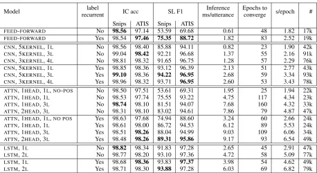
Table 1: Development results on the Snips 2017 and ATIS datasets, comparing models from feed-forward, convolutional, self-attention, and recurrent paradigms, as well as comparing non-recurrent, label-recurrent, and fully recurrent architectures, on IC, SL, inference speed, and training time. Inference speed, convergence time, and parameter count are drawn from Snips experiments, but the trends hold on ATIS. The best IC and SL for each dataset is bolded within each model paradigm to help compare between paradigms.
accuracy and SL F1. Second, we pick a small num-ber of our best-performing models to evaluate on ATIS and Snips test sets, to compare against prior work.
For each experiment below, we train until con-vergence, where convergence is defined by an early stopping criterion with a patience of 30 epochs and an average of development set IC ac-curacy and token-level SL F1 used as the perfor-mance metric.
6.1 Modeling study experiments
In our first category of experiments, we evaluate variants of each word contextualization paradigm introduced.
We evaluate one feed-forward word contextu-alization module (labeled asFEED-FORWARD) to
provide a baseline performance. As with all sub-sequent models, we evaluate this word contextu-alization module with and without our proposed label-recurrent decoder. This baseline should help us determine the extent to which each dataset re-quires the modeling of context.
We evaluate 3 convolutional word contex-tualization modules. The first has 1 layer with a kernel size of 5, and is intended to provide intuition as to whether a relatively large local
context can sufficiently model SL behavior. We label this model CNN, 5KERNEL, 1L, and name all other CNN models similarly. The next model has 3 layers with kernel size 5, and is dilated. This model incorporates long-distance context hierarchically, and is shorter and wider-per-layer than the otherwise-similar 3rd CNN model, with 4 layers and kernel size 3.
We evaluate 4 attention-based word contextual-ization modules. The first is simple, with 1 atten-tion head and 1 layer. Unlike all others we analyze, it does not use relative position embeddings. Thus, this model is word order-invariant except for a simple absolute position embedding. If it improves overFEEDFORWARD, then, it provides strong
evi-dence that semantic information from the context words, irrespective of order, is useful in making tagging decisions. We label this model with the flagNO-POS. To evaluate the utility of relative po-sition embeddings, we also compare a model with 1 head and one layer, labeled ATTN, 1HEAD, 1L. We then test two increasingly complex models, first with 3 layers and 1 head, the second with 3 layers and 2 heads per layer.
first. As with all other models, we test these two models both with independent slot prediction and label-recurrent slot prediction.
6.2 Comparison to prior work
For our second category of experiments, we take a few high-performing models from our analysis and evaluate them on the Snips and ATIS test sets for comparison to prior work. For these models, we report not only the average IC accuracy and SL F1 across random initializations, but also the stan-dard deviation and best model, as most work has not reported average values. We keep all hyperpa-rameters fixed across all experiments, potentially hindering performance but providing a stronger analysis of robustness.
Note on pre-trained contextual word embed-ding: Although our framework allows easy inte-gration of contextual pre-trained embeddings like BERT (Devlin et al., 2019) and EMLo (Gardner et al.,2017) by replacing the word contextualiza-tion component, we exclude them in our exper-imentation in order to reduce model obfuscation and have fair comparison against baselines.
7 Results and discussion
In this section, we draw from results reported in Table 1, on the development sets of Snips and ATIS. It is easy to see that very little in the way of modeling is necessary for IC task, so we focus our analysis on SL task. We emphasize that ATIS has shorter spans than Snips, averaging 1.2 and 1.8 tokens, respectively, leading to differing modeling requirements.
7.1 Minimal modeling for SLU
By analyzing three simple models - FEED
-FORWARD,ATTN-1HEAD-1L-NO-POS, andCNN
-5KERNEL-1L- we conclude that explicitly incor-porating local features is a useful inductive bias for high SL accuracy. The purely feed-forward model achieves 53.59 SL F1 on Snips, whereas one layer of convolution improves that number to 85.88. The story is similar for ATIS SL. How-ever, a single layer of attention without position information fails to improve over the feed-forward model whatsoever which we believe is due to the order-invariant nature of self-attention. This also emphasizes the fact that focusing on local context is useful inductive prior for SL task.
For each of these simple models, switching
from independent slot label prediction to label-recurrent prediction provides large gains on both datasets. We find an approximate 1.3ms/utterance slowdown from using label recurrence across all models. Thus, in terms of accuracy-for-speed, very simple models can achieve much of the results of more expensive models as long as they are label-recurrent and incorporate local context.
7.2 High-performing convolutional models
The larger convolutional models provide very high accuracy while maintaining fast inference and training speeds. In particular, our best CNN model, CNN-5KERNEL-3L, achieves 94.22 SL F1 on Snips, compared to the two-layer LSTM with label-recurrence, which achieves 93.88. The model achieves this modest improvement with over 2x the inference speed, training in under 1/2 the time, and demonstrating even stronger results on the test sets, discussed below.
On ATIS, where utterances are longer but slot label spans are shorter, LSTMs outperform CNNs on the development sets.
7.3 Issues with self-attention
Our strongest self-attention model underperforms CNNs and LSTMs on both Snips and ATIS, with a maximum SL of 89.31 and 95.86 on the datasets, respectively. Though self-attention models have seen success in complex tasks with lots of train-ing data, we suggest in this study that they lack the inductive biases to perform well on these small datasets.
Relative position embeddings go a long way in improving self-attention models; adding them to a 1-layer attentional encoder improves ATIS and Snips SL by approximately 24 and 22 points, re-spectively. We find that adding attention heads does not add considerably to the computational complexity of attention models, while increasing accuracy; thus in a speed-accuracy tradeoff, it is likely better to add heads rather than layers as each layer addsO(n2∗dx)additional computations.
7.4 Word and label recurrence in LSTMs
Snips
IC Acc SLR F1
Model Recurrence Mean Max Mean Max
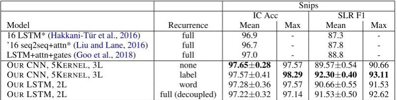
[image:8.595.97.502.62.164.2]16 LSTM* (Hakkani-T¨ur et al.,2016) full 96.9 - 87.3 -’16 seq2seq+attn* (Liu and Lane,2016) full 96.7 - 87.8 -LSTM+attn+gates (Goo et al.,2018) full 97.0 - 88.8 -OURCNN, 5KERNEL, 3L none 97.65±0.28 97.57 89.57±0.54 90.66 OURCNN, 5KERNEL, 3L label 97.57±0.41 98.29 92.30±0.40 93.11 OURLSTM, 2L word 97.28±0.36 97.57 90.66±0.55 91.53 OURLSTM, 2L full (decoupled) 97.22±0.32 97.14 91.53±0.50 92.62
Table 2: Test set results on the Snips dataset. (*) indicates numbers reported by (Goo et al.,2018)
ATIS
IC Acc SLR F1
Model Recurrence Mean Max Mean Max
[image:8.595.103.495.197.301.2]LSTM+attn+gates (Goo et al.,2018) full 94.10 - 95.20 -’18 Two LSTMs (Wang et al.,2018) full - 98.99 - 96.89 ’18 self-attn+LSTM (Li et al.,2018) full - 98.77 - 96.52 OURCNN, 5KERNEL, 3L none 97.04±0.62 97.98 94.84±0.22 94.95 OURCNN, 5KERNEL, 3L label 97.37±0.57 98.10 95.27±0.19 95.54 OURLSTM, 2L word 96.84±0.49 97.65 95.13±0.29 95.41 OURLSTM, 2L full (decoupled) 97.00±0.44 97.98 95.15±0.25 95.21
Table 3: Test set results on the ATIS dataset, compared to recent recurrent models.
7.5 Best models compared to prior work
We report test set results on Snips and ATIS in Tables2and3. Our best models from our valida-tion study,CNN-5KERNEL-3LandLSTM-2L,
out-perform the state-of-the-art on the Snips dataset, with label-recurrence proving crucial, especially for Snips. In particular, CNN-5KERNEL-3L with
label recurrence achieves an average SL F1 of 92.30, improving over the previous state-of-the-art of 88.8, by reducing error rate by 30%, and .57-point improvement on IC.
On ATIS, our label-recurrent models outper-form slot-gated LSTM model ofGoo et al.(2018) on both IC and SL tasks.3 Wang et al. (2018) attribute their result to using IC and SL-specific LSTMs and use 300-dimensional word embedding and 200-dimensional LSTMs, but with an ATIS vocabulary of 867 words (suggesting a relatively simple sequence space), we are unable to deter-mine the source of the improvement from a model-ing standpoint. Similar observation was made for (Li et al.,2018) where 264-dimension embeddings is used.
We hypothesize that our models perform bet-ter on Snips because much of Snips slot label-ing depends on consistency within long spans,
3
We note that, since this work was performed, consider-able efforts have been put into the Snips dataset, including the use of ELMo (Siddhant et al.,2019), BERT (Chen et al.,
2019b), and capsule networks (Zhang et al.,2019), among other methods (Chen et al.,2019a).
Figure 2: Visualization of the weight given to each token representation by the attention-based pooling for sentence representation. Lighter colors indicate greater attention.
whereas ATIS slot labels have longer-distance de-pendencies, for example between to city and from citytags.
7.6 Attention Visualization
We note that anecdotally, few words in each ut-terance are useful in indicating the intent. In the example given in Figure 2, presence of possible departure and arrival cities may be distracting, but the attention mechanism correctly learns to focus on words that indicateatis aircraftintent.
8 Conclusion
high performance in both accuracy and speed. With the results of this study, we proposed a convolution-based joint IC+SL model for SLU that achieves new state-of-the-art results on Snips dataset while maintaining a simple design, shorter training, and faster inference than comparable re-current methods.
9 Implementation details
All models are implemented in MXNet (Chen et al., 2015). For all models, we randomly ini-tialize word embeddings and use dx = 70. We
optimize using Adadelta algorithm (Zeiler,2012), with initial learning rate, .01. We clip and pad all training and development sentences to length 30, with clipping affecting a small number of ut-terances. Dropout (Srivastava et al., 2014) prob-ability of .3 is used in all models. We train us-ing a batch size of 128 split across 4 GPUs on a p3.8xlarge EC2 instance, and perform inference using CPUs on same machine.
Acknowledgements
We would like to thank the reviewers for their comments, as well as the Lex team at Amazon AI for helpful conversations and feedback.
References
Dzmitry Bahdanau, Kyunghyun Cho, and Yoshua Ben-gio. 2014. Neural machine translation by jointly learning to align and translate. ICLR.
Ivan Bilan and Benjamin Roth. 2018. Position-aware self-attention with relative positional encodings for slot filling. arXiv preprint arXiv:1807.03052.
Mengyang Chen, Jin Zeng, and Jie Lou. 2019a. A self-attention joint model for spoken language un-derstanding in situational dialog applications. arXiv preprint arXiv:1905.11393.
Qian Chen, Zhu Zhuo, and Wen Wang. 2019b. BERT for joint intent classification and slot filling. arXiv preprint arXiv:1902.10909.
Tianqi Chen, Mu Li, Yutian Li, Min Lin, Naiyan Wang, Minjie Wang, Tianjun Xiao, Bing Xu, Chiyuan Zhang, and Zheng Zhang. 2015. Mxnet: A flexible and efficient machine learning library for heteroge-neous distributed systems. InLearningSys at Neural Information Processing Systems 2015.
Kyunghyun Cho, Bart Van Merri¨enboer, Caglar Gul-cehre, Dzmitry Bahdanau, Fethi Bougares, Holger Schwenk, and Yoshua Bengio. Learning phrase rep-resentations using RNN encoder-decoder for statis-tical machine translation. InEMNLP.
Alice Coucke, Alaa Saade, Adrien Ball, Th´eodore Bluche, Alexandre Caulier, David Leroy, Cl´ement Doumouro, Thibault Gisselbrecht, Francesco Calta-girone, Thibaut Lavril, et al. 2018. Snips voice plat-form: an embedded spoken language understanding system for private-by-design voice interfaces. arXiv preprint arXiv:1805.10190.
Jacob Devlin, Ming-Wei Chang, Kenton Lee, and Kristina Toutanova. 2019. BERT: Pre-training of deep bidirectional transformers for language under-standing. InNAACL.
Matt Gardner, Joel Grus, Mark Neumann, Oyvind Tafjord, Pradeep Dasigi, Nelson F. Liu, Matthew Peters, Michael Schmitz, and Luke S. Zettlemoyer. 2017.AllenNLP: A deep semantic natural language processing platform.
Jonas Gehring, Michael Auli, David Grangier, Denis Yarats, and Yann N Dauphin. 2017. Convolutional sequence to sequence learning. In ICML, pages 1243–1252.
Chih-Wen Goo, Guang Gao, Yun-Kai Hsu, Chih-Li Huo, Tsung-Chieh Chen, Keng-Wei Hsu, and Yun-Nung Chen. 2018. Slot-gated modeling for joint slot filling and intent prediction. InProceedings of the 2018 Conference of the North American Chapter of the Association for Computational Linguistics: Hu-man Language Technologies, Volume 2 (Short Pa-pers), volume 2, pages 753–757.
Allen L Gorin, Giuseppe Riccardi, and Jeremy H Wright. 1997. How may i help you? Speech com-munication, 23(1-2):113–127.
D. Guo, G. Tur, W.T. Yih, and G. Zweig. 2014. Joint semantic utterance classification and slot filling with recursive neural networks. InProceedings of Spo-ken Language Technology Workshop (SLT), page 554–559.
Patrick Haffner, Gokhan Tur, and Jerry H Wright. 2003. Optimizing svms for complex call classification. In ICASSP, volume 1, pages I–I. IEEE.
Dilek Hakkani-T¨ur, G¨okhan T¨ur, Asli Celikyilmaz, Yun-Nung Chen, Jianfeng Gao, Li Deng, and Ye-Yi Wang. 2016. Multi-domain joint semantic frame parsing using bi-directional RNN-LSTM. In Inter-speech, pages 715–719.
C.T. Hemphill, J.J. Godfrey, and G.R. Doddington. 1990. The ATIS spoken language systems pilot cor-pus. InProceedings of the DARPA Speech and Nat-ural Language Workshop, page 96–101.
Sepp Hochreiter and J¨urgen Schmidhuber. 1997. Long short-term memory. Neural computation, 9(8):1735–1780.
Nikita Kitaev and Dan Klein. 2018. Constituency parsing with a self-attentive encoder. In Proceed-ings of the 56th Annual Meeting of the Association for Computational Linguistics (Volume 1: Long Pa-pers), pages 2676–2686. Association for Computa-tional Linguistics.
Changliang Li, Liang Li, and Ji Qi. 2018. A self-attentive model with gate mechanism for spoken lan-guage understanding. In Proceedings of the 2018 Conference on Empirical Methods in Natural Lan-guage Processing, pages 3824–3833.
B. Liu and I. Lane. 2016. Attention-based recurrent neural network models for joint intent detection and slot filling. InProceedings of Interspeech.
Robert E Schapire and Yoram Singer. 2000. Boostex-ter: A boosting-based system for text categorization. Machine learning, 39(2-3):135–168.
Peter Shaw, Jakob Uszkoreit, and Ashish Vaswani. 2018. Self-attention with relative position represen-tations. In Proceedings of the 2018 Conference of the North American Chapter of the Association for Computational Linguistics: Human Language Tech-nologies, Volume 2 (Short Papers), pages 464–468. Association for Computational Linguistics.
T. Shen, T. Zhou, G. Long, J. Jiang, S. Pan, and C. Zhang. 2017. DiSAN: Directional self-attention network for RNN/CNN-free language understand-ing.
Aditya Siddhant, Anuj Goyal, and Angeliki Metalli-nou. 2019. Unsupervised transfer learning for spo-ken language understanding in intelligent agents.
Nitish Srivastava, Geoffrey Hinton, Alex Krizhevsky, Ilya Sutskever, and Ruslan Salakhutdinov. 2014. Dropout: a simple way to prevent neural networks from overfitting. The Journal of Machine Learning Research, 15(1):1929–1958.
E. Strubell, P. Verga, D. Belanger, and A. McCallum. 2017. Fast and accurate entity recognition with iterated dilated convolutions. In Proceedings of EMNLP.
Ashish Vaswani, Noam Shazeer, Niki Parmar, Jakob Uszkoreit, Llion Jones, Aidan N Gomez, Łukasz Kaiser, and Illia Polosukhin. 2017. Attention is all you need. InAdvances in Neural Information Pro-cessing Systems, pages 5998–6008.
Yu Wang, Yilin Shen, and Hongxia Jin. 2018. A bi-model based RNN semantic frame parsing bi-model for intent detection and slot filling. In Proceed-ings of the 2018 Conference of the North American Chapter of the Association for Computational Lin-guistics: Human Language Technologies, Volume 2 (Short Papers), volume 2, pages 309–314.
P. Xu and R. Sarikaya. 2013. Convolutional neural net-work based triangular CRF for joint intent detection and slot labeling. In Proceedings of IEEE ASRU Workshop.
Kaisheng Yao, Baolin Peng, Yu Zhang, Dong Yu, Ge-offrey Zweig, and Yangyang Shi. 2014. Spoken lan-guage understanding using long short-term memory neural networks. In Spoken Language Technology Workshop (SLT), 2014 IEEE, pages 189–194. IEEE.
Fisher Yu and Vladlen Koltun. 2015. Multi-scale con-text aggregation by dilated convolutions. InICLR.
Matthew D Zeiler. 2012. Adadelta: an adaptive learn-ing rate method.arXiv preprint arXiv:1212.5701.
Chenwei Zhang, Yaliang Li, Nan Du, Wei Fan, and Philip S Yu. 2019. Joint slot filling and intent de-tection via capsule neural networks.