Maximum Likelihood Estimation of Factored Regular Deterministic
Stochastic Languages
Chihiro Shibata School of Computer Science
Tokyo University of Technology [email protected]
Jeffrey Heinz
Department of Linguistics &
Institute for Advanced Computational Science Stony Brook University
Abstract
This paper proves that for every class C of stochastic languages defined with the co-emission product of finitely many proba-bilistic, deterministic finite-state acceptors (PDFA) and for every data sequence D of finitely many strings drawn i.i.d. from some stochastic language, the Maximum Likelihood Estimate ofDwith respect toCcan be found efficiently by locally optimizing the parame-ter values. We show that a consequence of the co-emission product is that each PDFA be-haves like an independent factor in a joint dis-tribution. Thus, the likelihood function de-composes in a natural way. We also show that the negative log likelihood function is con-vex. These results are motivated by the study of Strictly k-Piecewise (SPk) Stochastic Lan-guages, which form a class of stochastic lan-guages which is both linguistically motivated and naturally understood in terms of the co-emission product of certain PDFAs.
1 Introduction
Stochastic languages are probability distributions over all possible strings of finite length. A class
C of stochastic languages is often defined para-metrically: an assignment of values to the parame-ters uniquely determines some stochastic language
L in C and thus the probabilities that L assigns to strings. An important learning criterion for a class of stochastic languagesCis whether there is an algorithm which reliably returns a Maximum-Likelihood Estimate (MLE) of an observed data sample D. The MLE is the parameter values which maximize the probability ofDwith respect toC.
This paper focuses on regular deterministic
stochastic languages. These are stochastic lan-guages that can be defined with a probabilistic, de-terministic, finite-state acceptors (PDFA).
The problem of finding the MLE, however, is not only about some single stochastic languageL, but also about the class of stochastic languages thatL belong to. It is well-understood that each PDFA M naturally defines a class of stochastic languages CM because the transitional probabil-ities in the PDFA provide a range of possible pa-rameter values, as we explain in detail in section2. In this case, it is well-understood how to find the MLE of a sequence of strings drawn i.i.d. fromL
with respect to CM (Vidal et al., 2005a,b). This paper is concerned with finding the MLE for dif-ferentclasses of stochastic languages.
In particular, we consider the case where C is defined by the range of parametric values over
finitely many PDFAA = {M1. . .MK}, whose co-emission product determines the probabilities eachL∈Cassigns to strings. Essentially, the co-emission product of these PDFAsfactorthe prob-abilities eachL∈C assigns to strings. EachLis a complex joint distribution, and each PDFAMj represents a ‘more basic’ regular stochastic lan-guage whose parameter values independently con-tribute toL. At a high level, the problem we are considering is like those addressed with Bayesian networks and Markov random fields, where com-plex probability distributions decompose into sim-pler factors (Bishop, 2006;Koller and Friedman,
2009). We refer to the classesC we study in this paper as factored, regular, probabilistic, and deter-ministic (FRPD).
There are several reasons for being interested in such factored classes C. Perhaps the most important from our perspective is expressed by Koller and Friedman (p. 1134) “The ability to exploit structure in the distribution is the basis for providing a compact representation of high-dimensional . . . probability spaces.” In our case, the size of the representation of the class given by A = {M1. . .MK}is simply the sum of the
size of each Mj. In contrast, the representation
of the class given by the co-emission product is in the worst case the product of the sizes of each
Mj. One direct benefit of this is that the number
of parameters is reduced, which makes it possible to more accurately estimate them with less data. Other advantages discussed by Koller and Fried-man, such as modularity, we return to in the dis-cussion in the conclusion.
There are also linguistic reasons to be interested in FRPD classes. The Strictly Piecewise (SP) class of languages encode certain types of long-distance dependencies found in natural languages. For ex-ample, SP languages can express generalizations like “at most one b per string” and “no b may fol-low an a” (Rogers et al., 2010). Generalizations with this formal character are known to occur in the phonologies of the world’s languages (Heinz,
2010a; Rogers et al., 2013; Heinz, 2014, 2018). AsRogers et al.(2010) explain, Strictly Piecewise languages are characterized by the intersection product of finitely many deterministic finite-state acceptors (DFA). Heinz and Rogers (2010) used this characterization and the co-emission product to define the class of Strictly Piecewise stochas-tic languages because they were interested in the learnability of long-distance dependencies in nat-ural languages probabilistically. They presented a learning algorithm for a class of SP stochastic languages and claimed (p. 894) that it returns the MLE.
This results in this paper can be seen as pro-viding a more generalized, more meaningful, and more rigorous proof of their basic claim. Theo-rem 2 establishes how to update the parametric values which locally optimize the model of any
FRPD class. Theorem 3 shows the negative log likelihood function ofanyFRPD class is convex, so there is in fact only one set of optimal para-metric values for any sequence of data. Further-more, we prove these results in terms of the stan-dard definition of co-emission product, and not the
variant used inHeinz and Rogers(2010). (While the results here work for both, we only prove the standard case.) These general results make it possible to explore not only the learning of SPk
stochastic languages, but alsoanyfinite combina-tion of PDFAs that characterize different kinds of local and non-local dependencies which can be ex-pressed with regular grammars. We return to this issue in the discussion.
To our knowledge, such results for FRPD classes have not been previously discussed in the literature. One reason for this is that much work on natural language processing uses probabilis-tic non-deterministic automata. These describe the same class of stochastic languages as Hidden Markov Models (HMMs) (Vidal et al., 2005a,b). Non-determinism can make a big difference when it comes to parsing and learning. In a determin-istic model M, each string w can be associated with at most one path through M, whereas in non-deterministicM, there can be infinitely many paths forw. This is one reason why methods used for learning HMM are not guaranteed to return a MLE. Since the states are ‘hidden’ one uses meth-ods like Expectation Maximization, which may converge to a local optimum that is not a global optimum (Jurafsky and Martin,2008;Heinz et al.,
2015).
On the other hand, we are showing that, by care-fully choosing the class of stochastic languages
C—which the MLE which is to be found will be ‘with respect to’—we can exploit the structure we assume to be present to guarantee we find a MLE. This paper takes one step in establishing the theo-retical soundness of this approach.
Finally, one reviewer commented that these results may follow from fundamental theorems in the literature on probabilistic graphical mod-els (Koller and Friedman, 2009). Regardless of whether this is true, the correctness of the proofs here stand. Also, the general results of Bayesian networks and Markov random fields say nothing about the concrete forms of the algorithm for ob-taining the MLE with respect to a FRPD classC
be made clear.
The remainder of the paper is organized as fol-lows. In section2we review languages, stochas-tic languages, determinisstochas-tic finite-state acceptors and probabilistic versions thereof, the intersection and co-emission products, and the statement of the learning problem. Before presenting our main re-sults, section3defines Strictly Piecewise (stochas-tic) languages, which provide a running example to illustrate the main results, which are presented in section4. The computational complexity of the updates are analyzed in section 5 and section 6
concludes.
2 Preliminaries
2.1 Sets of Strings
Σ denotes a finite set of symbols and Σk, Σ≤k, and Σ∗ denote all strings over this alphabet of length k, of length less than or equal to k, and of any finite length, respectively. λ denotes the empty string. The length of a stringw is written |w|. The prefixes of a string w are Pref(w) =
{v| ∃u∈Σ∗, vu=w}. A string w = σ1. . . σn
is a subsequence of a string v if and only if
v ∈ Σ∗σ1Σ∗. . .Σ∗σnΣ∗, in which case we write wvv.
A languageLis a subset of Σ∗. The comple-ment of a language L, denoted L is Σ∗/L. The
shuffle idealofwis the language of all strings con-tainingwas a subsequence:
SI(w) ={v|wvv}.
A stochastic language L is a probability dis-tribution over Σ∗. The probability P of wordw
with respect toLis writtenPL(w) =p. Thus, all
stochastic languagesLsatisfy
X
w∈Σ∗
PL(w) = 1.
2.2 Probabilistic Deterministic Finite-state Acceptors
A Deterministic Finite-state Acceptor (DFA) is a tuple M = hQ,Σ, q0, δ, Fi where Q is the
state set, Σ is the alphabet, q0 is the start state, δ is a deterministic transition function with do-main Q×Σ and codomain Q, and F is the set of accepting states. Let δ∗ : Q × Σ∗ → Q
be the (partial) path function of M. When dis-cussing partial functions, the notation↑ and↓ in-dicates that the function is not defined, respec-tively, is defined, for particular arguments. Thus
δ∗(q, w)is the (unique) state reachable from state
q via the sequence w, if any, or δ∗(q, w)↑ other-wise. The language recognized by a DFA Mis
L(M)def={w∈Σ∗ |δ∗(q0, w)↓ ∈F}.
A Probabilistic Deterministic Finite-state Ac-ceptor(PDFA) is a tupleM=hQ,Σ, q0, δ, F, Ti
whereQ,Σ, q0,andδ are the same as with DFA,
andFandT are partial functions representing the final-state and transition probabilities. In particu-lar,T :Q×Σ→R+andF :Q→
R+such that
for allq∈Q, F(q) +X σ∈Σ
T(q, σ) = 1. (1)
A PDFA M generates a stochastic language
L(M). If it exists, the uniquepathfor a wordw= σ0. . . σN belonging toΣ∗through a PDFA is a
se-quence h(q0, σ0),(q1, σ1), . . . , (qN, σN)i, where qi+1 =δ(qi, σi). The probability a PDFA assigns
towis obtained by multiplying the transition prob-abilities along w’s path if it exists with the final probability, and zero otherwise. SoPL(M)(w) =
N Y
i=0
T(qi, σi) !
·F δ(qN, σN)
ifδ∗(q0, w)↓and 0 otherwise (2)
A probability distribution isregular deterministic
iff there is a PDFA which generates it. We some-times writeM(w)instead ofPL(M)(w).
The structural components of a PDFA Mare its statesQ, its alphabetΣ, its transitionsδ, and its initial stateq0. Bystructureof a PDFA, we mean
its structural components. The structure of each PDFAMdefines a class of stochastic languages given by the possible instantiations of T and F
satisfying Equation1. These distributions have at most|Q|·(|Σ|+ 1)independent parameters (since for each state there are|Σ|possible transitions plus the possibility of finality.)
2.3 The co-emission product
Theintersection productofKDFAsM1. . .MK is given by the standard construction over the state space Q1 × . . . × QK (Hopcroft et al., 2001). We write N
1≤j≤KMj = M =
hQ,Σ, q0, δ, Fi where Q = Q1 × . . . × QK, q0 = hq01, . . . q0Ki. For allhq1, . . . qKi ∈ Qand σ ∈ Σ, δ(hq1, . . . qKi, σ) = hq01, . . . qK0 i if and
only ifδ1(q1, σ) = q01, . . .δK(qK, σ) = q0K.
Fi-nally, letF =F1×. . .×FKIt is well-known that L(N
The co-emission product of K PDFAs M1. . .MK is also given by a construction over
the state space Q1 ×. . . ×QK. The
probabil-ity that σ is co-emitted from hq1, . . . , qKi in Q1 × . . .] × QK is the product of the
proba-bilities of its emission at each qj ∈ Qj. Let
CoT(hσ, q1 . . . qKi) = QKj=1Tj(qj, σ).
Simi-larly, the probability that a word simultaneously ends atq1 ∈Q1, . . . qK ∈QKis
CoF(hq1 . . . qKi) = K Y
j=1
Fj(qj).
Finally, forq=hq1 . . . qKi, let Z(q) =CoF(q) + X
σ∈Σ
CoT(hσ, qi)
be thenormalization term. Next we define the co-emission product.
Definition 1 (Co-emission Product) For A =
{M1, . . .MK}, let NA = hQ,Σ, q0, δ, F, Ti where
1. Q, q0,andδare defined as with DFA product; and
2. For allq∈Qandσ∈Σ:
F(q) = CoF(q) Z(q)
and
T(q, σ) = CoT(σ, q) Z(q) .
In other words, the numerators ofT andF are de-fined to be the co-emission probabilities and divi-sion byZ ensures that co-emission productNA
defines a well-formed probability distribution over
Σ∗.
Observe thatAalso defines a class of stochas-tic languages by the possible instantiations ofTj
andFj for eachMj ∈ A. The structural compo-nents of Aare the structural components of each
Mj ∈ A. By structure ofA, we mean its struc-tural components. The structure of A defines a class of stochastic languages given by the possible instantiations of Tj andFj satisfying Equation 1
for eachMj ∈ A. If NA
= Mthen the class of stochastic lan-guages induced by the structure ofAis a subset of the class of stochastic languages obtained with the structure of the PDFAM. This is another way of saying that a factorized model may have fewer pa-rameters and so the class of stochastic languages it represents can become smaller.
2.4 Statement of the Learning Problem
LetDbe a finite sequence of|D|i.i.d. drawn ex-amples from a stochastic language L. It follows that thePL(D) =Qw∈DPL(w).
LetA={M1. . .MK}be a set of PDFAs and
let CA denote the FRPD class of stochastic lan-guages induced by the structure ofA. The likeli-hoodofDw.r.t. CAis determined by the param-eters (theTj andFj functions for eachMj ∈ A).
Let us group these parameters under the symbol
Θ. Each Θ identifies some stochastic language
LΘ ∈ CA. Thelikelihood ofD w.r.t. CA is de-fined as follows:
lhd(D|Θ) = Y w∈D
PLΘ(w).
The problem of finding a Maximum Likelihood Estimate (MLE) is to find those parameter values
ˆ
Θ ofA that maximize the likelihood of D w.r.t.
CA. Formally,
ˆ
Θ = arg max Θ
lhd(D|Θ)
(3)
whereΘunder thearg maxranges over all possi-ble parameter values ofA.
When |A| = 1 the problem has a known so-lution. As mentioned, a single PDFAMdefines a class of stochastic languages given by possible parameter values of M. In this case, it is well-known how to findΘˆ. Essentially, each transition probability T(q, σ) equals the relative frequency that symbolσ is emitted at a stateq (Vidal et al.,
2005a,b). In this paper, we solve this problem when|A|>1.
3 Strictly k-Piecewise stochastic languages
In this section, we introduce the Strictly k -Piecewise stochastic languages, which serve as a running example of a FRPD class in the remain-der of the paper.
Rogers et al.(2010) define and provide multiple characterizations of Strictly Piecewise (SP) lan-guages. We review the most relevant ones for this paper here. SP languages are exactly those formal languages that are closed under subsequence.
SP= {L⊆Σ∗| ∀w, v∈Σ∗
(v∈L, wvv⇒w∈L)}
stringsSsuch thatLis the intersection of the com-plements of the shuffle ideals ofS.
Theorem 1 ∀L ∈SP,∃S ⊆Σ∗, n∈Nsuch that
|S|< nandL=T
w∈SSI(w).
The SP languages are parameterized by a value
k ∈ N. This number corresponds to the length of the longest string in S. For each SP language
L, if there is a setS whose longest string is equal tok, thenLbelongs to the SPkclass of languages.
If k is known a priori then the SPk languages
are both PAC-learnable and identifiable in the limit in polynomial time and data (Heinz,2010b;Heinz et al.,2012).1
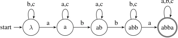
Theorem 1 allows one to construct concrete computational models for SP languages with DFA. For any nonempty stringw=σ1. . . σn,SI(w) = L(Mw) where Mw is defined as follows. The states are the prefixes ofw, the start state isλ, and the final state is w. For all prefixes p ofw and
σ ∈ Σ, letδ(p, σ) = pσwheneverpσis a prefix ofwandpotherwise. Figure1gives an examples of DFA forMabba.
The complementSI(w)is essentially obtained fromMwby removing its maximal state and
mak-ing every state final. In other words, if w = va
then theSI(w)can be recognized by an automa-ton where the states are the prefixes ofv, the start state is λ, and each state is a final state. For all prefixespofvandσ∈Σ,δ(p, σ) =pσwhenever
pσis a prefix of v. When pσis not a prefix of v
andσ 6= athen δ(p, σ) = p. Finally, δ(v, a) is not defined. We denote such a DFA asMw.
Fig-ure2shows the DFAMabba which recognizes the complement ofSI(abba). BothMwand the DFA recognizing its complement are minimal.
It follows that for anyL∈SP, one can construct a DFA recognizing L by taking theproductof the complements of the shuffle ideals of the strings in
S.
Note the size of M1. . .MK is P
1≤i≤KMj
whereas the size of M = N
1≤j≤KMj is in
the worst caseQ
1≤j≤KMj. Therefore, to decide
whether a stringw belongs to some SP language
L, it may be preferable to runw on eachMj
in-stead of on M to avoid the potentially large
in-1
Also, SP languages suggest a different representation for strings (Rogers et al.,2013), which inform machine learning in other ways. The winning paper of the SPiCE competition (Balle et al.,2016), in which machine learning models com-peted to best predict the next symbol in a natural and artificial sequences was won byShibata and Heinz(2016), who inte-grated SP-style representations into a neural network.
crease in the state space. See Heinz and Rogers
(2013) for additional discussion of this point.
Heinz and Rogers (2010) use the fact that SP languages are the intersection of the comple-ments of shuffle ideals to define their stochastic counterpart. They define stochastic versions of Mw (Figure 2), which they call w-subsequence-distinguishing PDFA.
Definition 2 (Subsequence-distinguishing PDFA)
Let w ∈ Σk−1 and w = σ1· · ·σk−1.
Mw = hQ,Σ, q0, δ, F, Ti is a
w-subsequence-distinguishing PDFA (w-SD-PDFA) iff F and T satisfy Equation 1 and δ(u, σ) = uσ whenever uσ∈Pref(w)anduotherwise.
Apart from the stochastic components T andF, the w-subsequence-distinguishing PDFA differs from Mw in one key way. Suppose. w = va. Then δ(v, a) = v in the w -subsequence-distinguishing PDFA is not undefined as was the case with Mw. This transition exists and may have a nonzero probability.
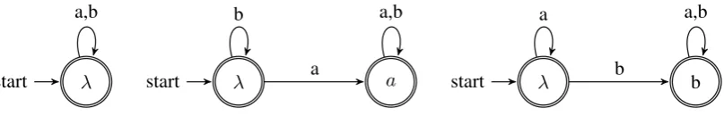
A set Aof PDFAs isak-set of SD-PDFAsiff, for eachw ∈ Σ≤k−1, it contains exactly one w -SD-PDFA. For example, letΣ = {a, b}and con-sider the 2-set of SD-PDFAs shown in Figure 3. There are three SD-PDFAs in this set correspond-ing toMλ,Ma, andMb.
Heinz and Rogers(2010) define SPk stochastic
languages as a product of a k-set of SD-PDFAs. Specifically, the adapt the notion of co-emission probability (Vidal et al.,2005a).Heinz and Rogers
(2010) actually use what they call thepositive co-emission productwhich restricts the standard co-emission probability to particular circumstances.
In this work, we define SP stochastic languages with the standard definition ofco-emission proba-bilityused to define products of PDFA as in Defi-nition1(Vidal et al.,2005a).
Definition 3 (SP Stochastic Languages) A prob-ability distributionP over Σ∗ is a SP stochastic language iff there exists ak-set of SD-PDFAsA, whose co-emission product is M = N
A, such that for all w ∈ Σ∗, it is the case thatP(w) =
M(w).
be-λ
start a a ab abb abba
b,c
b a,c
b a,c
a
[image:6.595.153.449.69.132.2]b,c a,b,c
Figure 1: The DFAMabbaforSI(abba)(left) withΣ ={a, b, c}.
λ
start a a ab abb
b,c
b a,c
b
a,c b,c
Figure 2: The DFAMabbaforSI(abba)withΣ ={a, b, c}.
cause there are three actions associated with each state (a, b, and finality); there are five states; but since the probabilities must add to one only two parameters per state are free. More generally, a
k-set of SD-PDFAs A has |Σ| · P
j∈A|Qj| free
parameters.
4 Main Theorem for MLE of FRPD classes
We provide our main results here, using the 2-set of SD-PDFAs shown in Figure3as an illustrative example.
4.1 The Co-emission Probability Given a Prefix
It is useful to consider the co-emission probabil-ity of the symbol σ given the prefix σ1· · ·σi−1,
which we denote Coemit(σ, i). It follows from Definitions1 and3that this value is the normal-ized product of the path through N
A given by the prefixσ1· · ·σi−1.
Formally, let M1 = hQ1,Σ, q01, δ1, F1, T1i,
· · ·,MK =hQK,Σ, q0K, δK, FK, TKibe exactly
those PDFAs inA. Suppose thatw = σ1· · ·σN,
where σi ∈ Σ for all 1 ≤ i ≤ N. Let q(j, i)
denote a state in Qj that is reached after Mj
reads the prefixσ1· · ·σi−1. If i = 1thenq(j, i)
represents the initial state of Mj. Then it
fol-lows from Definition 1 that the probability that a symbol σ is emitted after the product machine
N
1≤j≤KMj reads the prefix σ1· · ·σi−1 is the
following:Coemit(σ, i) =
QK
j=1Tj(q(j, i), σ) P
σ0∈Σ
QK
j=1Tj(q(j, i), σ0
+QKj=1Fj(q(j, i))
(4)
To simplify the notation and analysis, we as-sume that there is a end marker n ∈ Σ which
uniquely occurs at the end of words. This lets us replaceFj(q)withTj(q,n). ThenCoemit(σ, i)is
simply written as
Coemit(σ, i) =
QK
j=1Tj(q(j, i), σ) P
σ0∈ΣQKj=1Tj(q(j, i), σ0). (5) The probability that the machineN
1≤j≤KMj
ac-ceptsw is obtained by taking the product of the co-emission probabilities for alli:
P(wn) = N+1
Y
i=1
Coemit(σi, i), (6)
whereσN+1=n.
Since we are concerned with the co-emission probabilities, which is a ratio, it is notewor-thy that in fact it does not matter if the sum
P
σ0∈ΣTj(q, σ0)is 1. The ratioCoemit(σ, i) and thusP(wn)are invariant with respect to the scale
ofTj(q, σ0) and the sumP
σ0∈ΣTj(q, σ0). Writ-ing this last value asz(j, q), it can easily be con-firmed by the fact that multiplying both the de-nominator and the numerator by 1/z(j, q) does not change the value of Coemit(σ, i) while nor-malizing Tj(q,·). Thus, we can relax the
condi-tion in Equacondi-tion 1 when discussing co-emission probabilities. The only condition that needs to be satisfied with respect to the transitions is that
Tj(q, σ0) ≥ 0 for all j, q, σ0. Note that relaxing
[image:6.595.183.420.169.232.2]λ
start start λ a start λ b
a,b
a
b a,b
b
[image:7.595.101.505.64.129.2]a a,b
Figure 3: The 2-set of of SD-PDFAs withΣ ={a, b}.
4.2 Frequency and Empirical Mean of Co-emission Probability
Before describing the main theorem, we define two terms; the frequency of an emission and
the empirical mean of a co-emission probability, which play important roles in estimating transition probabilities for product machines.
Definition 4 (Frequency of Emission) For given w, we define the frequency ofσatq ∈ Qj as fol-lows. Let
• mw(Mj, q, σ)∈Z+denotes how many times σis emitted at the stateq while the machine Mjemitsw.
• nw(Mj, q) ∈ Z+ denotes how many times the state q is visited while the machine Mj emitsw.
Then
freqw(σ|Mj, q) = mw(Mj, q, σ)
nw(Mj, q) , (7)
So freqw(σ|Mj, q) represents the relative
fre-quency that Mj emits σ at q during emission of
w.
These concepts can be lifted to a sequence of stringsD drawn i.i.d. from some stochastic lan-guage. Let
mD(Mj, q, σ) = X
w∈D
mw(Mj, q, σ)
and
nD(Mj, q) = X
w∈D
nw(Mj, q).
It follows that
freqD(σ|Mj, q) =
mD(Mj, q, σ) nD(Mj, q)
.
So freqD(σ|Mj, q) represents the relative fre-quency that Mj emits σ at q during emission of D.
As an example, consider the 2-set of PDFAs in Figure 3 and consider the sample data D =
habbn, abani. Figure4shows the paths of these
strings through each SD-PDFA. Figure 5 shows some of the frequency computations.
If K = 1, i.e., the product machine consists of one PDFA thenfreqw(σ|M1, q)is the MLE of T1(q, σ) (Vidal et al., 2005a,b). Meanwhile, if K ≥ 2, the probability of the emission, which equals the co-emission probability, fluctuates with states that other machines are currently at. Thus
freqw(σ|Mk, q), as a random variable, is not inde-pendent from other machines’ states. This moti-vates the following definition.
Definition 5 (Empirical Mean) Let
sumCoemitw(σ, Mj, q) =
X
is.t.q(j,i)=q
Coemit(σ, i).
Theempirical mean of a co-emission probability
is defined as follows:
Coemitw(σ|Mj, q) =
sumCoemitw(σ, Mj, q) nw(Mj, q) ,
(8)
i.e., the sample average of the co-emission proba-bility whenq ∈Qj is visited.
When a state in Mj is visited more than once while emittingw, it does not imply that some other state in Mh is also visited more than once. In
other words, if there are positionsi6= `such that
q(j, i) =q(j, `)then it does not have to follow that
q(h, i) = q(h, `) for another machineMh. Thus,
even when Mj and the value ofq(j, i) are fixed,
Coemit(σ, i)fluctuates. The empirical mean is the average taken over such fluctuating co-emission probabilities.
4.3 Main Theorem and Convexity
Theorems 2and3are our main results. We sim-plify the proofs by assuming that D consists of a single sentence. That is, in both theorems, we consider D = {wn}. We can do this
Mλ: λ a λ b λ b λ n λ b λ b λ b λ n
Ma: λ a a a λ λ λ λ
a b b n b b b n
[image:8.595.112.479.63.135.2]Mb: λ a λ b b b b n λ b b b b b b n
Figure 4: The paths of{abbn,bbbn}through the 2-set of of SD-PDFAs withΣ ={a, b}.
freqD(a|Mλ, λ) = 1/8 freqD(a|Ma, λ) = 1/5 freqD(a|Ma, a) = 0/3,
freqD(b|Mλ, λ) = 5/8 freqD(b|Ma, λ) = 3/5 freqD(b|Ma, a) = 2/3,
freqD(n|Mλ, λ) = 2/8 freqD(n|Ma, λ) = 1/5 freqD(n|Ma, a) = 1/3,
freqD(a|Mb, λ) = 1/3 freqD(a|Mb, b) = 3/5,
freqD(b|Mb, λ) = 2/3 freqD(b|Mb, b) = 0/5,
[image:8.595.81.537.357.769.2]freqD(n|Mb, λ) = 0/3 freqD(n|Mb, b) = 2/5,
Figure 5: Frequency computations withD={abbn,bbbn}and the 2-set of of SD-PDFAs in Figure4.
without changing the probability of its production. To see why, we can adjust the transition func-tion of each PDFA Mj so that δj(q,n) = q0j
for each q ∈ Qj. In other words, once n is
emitted, the machines reset to their start states. Then for any D = {w1n,· · · , wkn}, we have P(D) = P(concat(D)) where concat(D) = w1nw2n· · ·nwkn. Thus, wnin both
theo-rems can be understood asconcat(D).
Theorem 2 Suppose that P(wn) is defined as Equation 6 for a product machine N
1≤j≤KMj and a wordw. Then,∂P(wn)/∂Tj = 0holds for alljif and only if the following equation is satis-fied for all1≤j≤K:
freqw(σ|Mj, q) =Coemitw(σ|Mj, q).
From Theorem 3, it will then follow that
T1, . . . TK are the MLE.
ProofBy taking the log of Eq.6, we have
logP(wn) = N+1
X
i=1
K X
j=1
logTj(q(j, i), σi)
−log X σ0∈Σ
K Y
j=1
Tj(q(j, i), σ0)
= N+1
X
i=1 K X
j=1
logTj(q(j, i), σi)
−
N+1 X
i=1
log X σ0∈Σ
K Y
j=1
Tj(q(j, i), σ0).
We differentiate this by a log emission probabil-itylogTh(q, σ)for some1≤h≤K. Let
A= ∂
∂logTh(q, σ) N+1
X
i=1 K X
j=1
logTj(q(j, i), σi),
and
B = ∂
∂logTh(q, σ) N+1
X
i=1
logX σ0∈Σ
K Y
j=1
Tj(q(j, i), σ0).
Then
∂ ∂logTh(q, σ)
logP(wn) =A−B.
First, we calculateA. Since
∂Tj(q(j, i), σi) ∂logTh(q, σ) =
1 ifhMh, q, σi
=hMj, q(j, i), σii, 0 otherwise,
we have
A= N+1
X
i=1 K X
j=1
I
hMh, q, σi=hMj, q(j, i), σii
= N+1
X
i=1
I
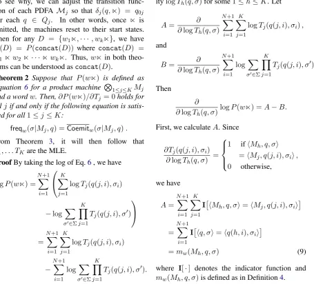
hq, σi=hq(h, i), σii
=mw(Mh, q, σ) (9)
where I[·] denotes the indicator function and
B = ∂ ∂logTh(q, σ)
N+1 X
i=1 log
X
a∈Σ K Y
j=1
Tj(q(j, i), a)
= N+1
X
i=1 ∂ ∂logTh(q,σ)
P a∈Σ
QK
j=1Tj(q(j, i), a) P
a∈Σ QK
j=1Tj(q(j, i), a)
= N+1
X
i=1 ∂ ∂logTh(q,σ)
P
a∈Σexp PK
j=1logTj(q(j, i), a)
P a∈Σ
QK
j=1Tj(q(j, i), a)
= N+1
X
i=1 P
a∈Σ
exp PKj=1logTj(q(j, i), a) PKj=1 ∂logTh(q(j,i),a)
∂logTh(q,σ)
P a∈Σ
QK
j=1Tj(q(j, i), a)
= N+1
X
i=1 P
a∈Σ
QK
j=1Tj(q(j, i), a)PKj=1
∂logTj(q(j,i),a)
∂logTh(q,σ)
P a∈Σ
QK
j=1Tj(q(j, i), a)
= N+1
X
i=1 X
a∈Σ
QK
j=1Tj(q(j, i), a) P
b∈Σ QK
j=1Tj(q(j, i), b) K X
j=1
∂logTj(q(j, i), a) ∂logTh(q, σ)
Figure 6: Initial calculation of B in the proof of Theorem2.
Second, we calculate B as shown in Figure6. There are two large terms in the large parentheses in the last line of the calculation of B in Figure6. The first one is is the co-emission probability by Equation5. Thus B =
N+1 X
i=1 X
a∈Σ K X
j=1
Coemit(a, i)∂logTj(q(j, i), a) ∂logTh(q, σ)
.
Recall that
∂logTj(q(j, i), a) ∂logTh(q, σ)
equals
I[hMh, q, σi=hMj, q(j, i), ai].
This indicator function equals I[h = j]I[q = q(j, i) ]I[σ = a]. Abbreviating I[h = j]with
I1,I[q =q(j, i) ]withI2, and I[σ = a]withI3,
we see that
X
a∈Σ K X
j=1
Coemit(a, i)I1I2I3
= K X
j=1
Coemit(σ, i)I1I2
=Coemit(σ, i)I[q=q(h, i)].
We conclude that
B = N+1
X
i=1
Coemit(σ, i)I[q=q(h, i)]
= X
is.t.q(h,i)=q
Coemit(σ, i)
=sumCoemitw(σ, Mh, q). (10)
By plugging our calculations of A (Eq. 9) and B (Eq.10) intoA=Band dividing the both sides bynw(Mh, q), we obtain the result
freqw(σ|Mh, q) =Coemitw(σ|Mh, q)
from the definitions of the relative frequency of an emission (Eq.7) and the empirical mean of a co-emission probability (Eq. 8). This concludes
the proof of Theorem2.
Next we prove that maximizingP(w)is a con-vex optimization problemto ensure that the solu-tion is the maximum point.
Following Boyd and Vandenberghe (2004), A set of points C inRnisconvexif the line segment
between any two points in C also lies in C. For-mally, C is convex provided for any x1, x2 ∈ C
the domain off is a convex set and if for allx, y
in the domain off, andtwith0≤t≤1, we have
f(tx+ (1−t)y)≤tf(x) + (1−t)f(y). We say
f isconcaveif−f is convex.
Recall from section2.4that the likelihood of a sequence of dataDto a stochastic languageL be-longing to a class with parameters Θ is lhd(D |
Θ) =Q
w∈DPL(w). The likelihood function is a
functionf : Rn → Rwheren is the number of
parameters|Θ|.
Let τj,q,σ denote logTj(q, σ); i.e. the log of some parameter in Θ. There are n =
|Σ|PKj=1|Qj| parameters in Θ since σ ∈ Σ, 1≤j≤K, andq ∈Qj. Thisτ can be thought of as a vector inRn.
The problem of maximizingP(wn)is the same
as minimizing −logP(wn) as a function of τ.
We show thatlogP(wn) is concave with respect
tologTj(q, σ) (Theorem3). If so, it is true that
the solution shown in Theorem2is a global max-imum.
Theorem 3 logP(wn)is concave with respect to τ ∈Rn.
Proof By taking the log of Eq. 6 , we have
logP(wn) =
N+1 X
i=1
K X
j=1
logTj(q(j, i), σi)
−logX a∈Σ
K Y
j=1
Tj(q(j, i), a)
.
Substituting inτ, it follows thatlogP(wn) =
N+1 X
i=1
K X
j=1
τj,q(j,i),σi−logX a∈Σ
K Y
j=1
exp(τj,q(j,i),a)
.
Since
K Y
j=1
exp(τj,q(j,i),a) = exp K X
k=1
τk,q(j,i),a !
,
and by letting ga(τ) = Pjτj,q(j,i),a, we obtain logP(wn) =
N+1 X
i=1
gσi(τ)−log
X
a∈Σ
exp (ga(τ)) !
.
Generally speaking, a composition f(x) = h(g1(x),· · · , gk(x))obeys the following rule: f
is convex if h is convex, h is non-decreasing in each argument, and gi is convex (see vector composition in Boyd and Vandenberghe, 2004, section 3.2.4)). Furthermore, it is known that
logP
exp(·) is convex (see section 3.1.5), and
logP
exp(·)is non-decreasing in each argument since both exp(·) and log(·) are non-decreasing. In addition,ga(·)is both convex and concave since every linear function is so from the definition (see section 3.1.1). Thus,logP
aexp(ga(·))is convex,
and−logP
aexp(ga(·))is concave.
Finally, from the fact that non-negative weighted sum preserves convexity and concavity (Boyd and Vandenberghe, 2004, section 3.2.1),
logP(wn)is concave.
It follows that the negative log ofP(wn)is
con-vex.
It is noteworthy to point out that establishing concavity does not mean the solution is unique. In fact, the solutions can be a set of points. An exam-ple FRPD class illustrating this is one which con-tains two PDFAM1andM2with the same struc-ture. For example suppose each had exactly one state with self-loop transitions for every symbol in
Σ. The co-emission productM1NM
2 does not
uniquely factorize though the above theorem es-tablishes its convexity.
Of course it is also of interest to know when the solution is unique. In this case, we have to show the negative log probability is strictly convex ex-cept for multiplying the emission probability by a constant. We leave this as an area of future re-search.
5 Optimization and Time Complexity
In this section, we discuss the time complexity and also how to optimize. From the proof of Theo-rem2, we have the following fact immediately.
Corollary 1 The update equation for max-imization of logP(wn) is represented as:
logTj(q, σ) :=
logTj(q, σ) +η(freqw(σ|Mj, q)
−Coemitw(σ|Mj, q)
(11)
if the simplest gradient method is applied, and where η is the step size. The time complexity for each update isO(N K|Σ|).
The time complexity for freqw(σ|Mj, q) and
Coemitw(σ|Mj, q) are shown in Lemma 1
Coemitw(σ|Mj, q) is a little higher than that of
freqw(σ|Mj, q).
Lemma 1 For all Mj and q ∈ Qj, freqw(σ|Mj, q) are computed in the time O(N K).
Proof We trace all machines while they are emitting σ1,· · ·, σN. Suppose that machines
are at q(1, i),· · · , q(K, i) after σ1,· · ·, σi−1
are emitted sequentially. For each step i, for all machinesMj, we have to update the counting for the pair of q(k, i) and σi, in order to calculate mw(Mj, q, σ). So the computational cost for each
stepiisO(K).
Lemma 2 For all Mj and q ∈ Qj,
Coemitw(σ|Mj, q) are computed in the time O(N K|Σ|).
Proof We trace all machines while they are emitting σ1,· · ·, σN. Suppose that machines
are at q(1, i),· · · , q(K, i) after σ1,· · ·, σi−1
are emitted sequentially. The critical part is calculating sumCoemit(σ)hMj,qi(w) . For each
step i, we have to update emission probabilities for all pairs ofMj andσ ∈ Σ. This update is in the timeO(K|Σ|). Thus, the time complexity for calculatingsumCoemitw(σ, Mj, q)isO(N K|Σ|).
6 Conclusion
The negative log likelihood function associated with a FRPD class C is convex, and it is pos-sible to efficiently find a MLE of any sequences of data generated i.i.d. with respect to C. Es-sentially, the parameters of the model are found by running the corpus through each of the indi-vidual factor PDFAs and calculating the relative frequencies. While this was the approach adopted byHeinz and Rogers(2010) for SP stochastic lan-guages, we have generalized it to sets of finitely many PDFAs.
There are several directions for future research, both theoretical and applied. On the theoretical side, one clear avenue is to better understand these results in terms of probabilistic graphical mod-els (Koller and Friedman, 2009). As a reviewer pointed out, the application of those methods to formal language theory and grammatical inference (de la Higuera,2010) appears fruitful.
On the applied side, there are several different opportunities. One area of interest is language modeling. The results here permit a modular ap-proach to constructing language models, where certain primitive factors are included or excluded. For example, we expect that language models which incorporate both n-gram models (Jurafsky and Martin, 2008) (which cannot describe long-distance dependencies) and SP stochastic lan-guages (which can describe some kinds of long-distance dependencies) will have lower perplex-ity, a hypothesis under current investigation. More generally, researchers can use aspects of the sub-regular hierarchies of languages (Thomas, 1997;
Rogers et al.,2013) to identify a range of ‘primi-tive factors’ whose DFA models can form the basis of various FRPD classes.
Finally, we are also interested in extending these results to weighted deterministic automata for computing regular relations (Beros and de la Higuera, 2016) or elements of other monoids (Gerdjikov,2018).
Acknowledgments
We would like to thank two anonymous reviewers for helpful comments, and another anonymous re-viewer in particular for making clear the scope of this work, which resulted in a significant revisions to our original submission. This work was sup-ported by NIH grant #R01HD87133-01 to JH and JSPS KAKENHI grant #JP18K11449 to CS.
References
Borja Balle, R´emi Eyraud, Franco M. Luque, Ariadna Quattoni, and Sicco Verwer. 2016. Results of the se-quence prediction challenge (SPiCe): a competition on learning the next symbol in a sequence. In Pro-ceedings of The 13th International Conference on Grammatical Inference, volume 57 ofJMLR: Work-shop and Conference Proceedings, pages 132–136.
Achilles Beros and Colin de la Higuera. 2016. A canonical semi-deterministic transducer. Funda-menta Informaticae, 146(4):431–459.
Christopher M. Bishop. 2006. Pattern Recognition and Machine Learning. Information Science and Statis-tics. Springer.
S. Boyd and L. Vandenberghe. 2004. Convex optimiza-tion. Cambridge.
of (sub)sequential transducers. InLanguage and Au-tomata Theory and Applications - 12th International Conference, LATA 2018, Ramat Gan, Israel, April 9-11, 2018, Proceedings, pages 143–155.
J. Heinz and J. Rogers. 2010. Estimating Strictly Piecewise Distributions. Proceedings of the 48th Annual Meeting of the Association for Computa-tional Linguistics, pages 886–896.
Jeffrey Heinz. 2010a. Learning long-distance phono-tactics. Linguistic Inquiry, 41(4):623–661.
Jeffrey Heinz. 2010b. String extension learning. In Proceedings of the 48th Annual Meeting of the As-sociation for Computational Linguistics, pages 897– 906, Uppsala, Sweden. Association for Computa-tional Linguistics.
Jeffrey Heinz. 2014. Culminativity times harmony equals unbounded stress. In Harry van der Hulst, editor,Word Stress: Theoretical and Typological Is-sues, chapter 8. Cambridge University Press, Cam-bridge, UK.
Jeffrey Heinz. 2018. The computational nature of phonological generalizations. In Larry Hyman and Frans Plank, editors, Phonological Typology, Pho-netics and Phonology, chapter 5, pages 126–195. De Gruyter Mouton.
Jeffrey Heinz, Colin de la Higuera, and Menno van Zaanen. 2015. Grammatical Inference for Compu-tational Linguistics. Synthesis Lectures on Human Language Technologies. Morgan and Claypool.
Jeffrey Heinz, Anna Kasprzik, and Timo K¨otzing. 2012. Learning with lattice-structured hypothesis spaces. Theoretical Computer Science, 457:111– 127.
Jeffrey Heinz and James Rogers. 2013. Learning sub-regular classes of languages with factored determin-istic automata. InProceedings of the 13th Meeting on the Mathematics of Language (MoL 13), pages 64–71, Sofia, Bulgaria. Association for Computa-tional Linguistics.
Colin de la Higuera. 2010. Grammatical Inference: Learning Automata and Grammars. Cambridge University Press.
John Hopcroft, Rajeev Motwani, and Jeffrey Ullman. 2001.Introduction to Automata Theory, Languages, and Computation. Boston, MA: Addison-Wesley.
Daniel Jurafsky and James Martin. 2008. Speech and Language Processing: An Introduction to Natu-ral Language Processing, Speech Recognition, and Computational Linguistics, 2nd edition. Prentice-Hall, Upper Saddle River, NJ.
Daphne Koller and Nir Friedman. 2009. Probabilistic Graphical Models: Principles and Techniques. MIT Press.
Robert Malouf. 2002. A comparison of algorithms for maximum entropy parameter estimation. In Pro-ceedings of the 6th Conference on Natural Language Learning - Volume 20, COLING-02, pages 1–7. As-sociation for Computational Linguistics.
James Rogers, Jeffrey Heinz, Gil Bailey, Matt Edlef-sen, Molly Visscher, David Wellcome, and Sean Wibel. 2010. On languages piecewise testable in the strict sense. InThe Mathematics of Language, vol-ume 6149 ofLecture Notes in Artifical Intelligence, pages 255–265. Springer.
James Rogers, Jeffrey Heinz, Margaret Fero, Jeremy Hurst, Dakotah Lambert, and Sean Wibel. 2013. Cognitive and sub-regular complexity. In Formal Grammar, volume 8036 ofLecture Notes in Com-puter Science, pages 90–108. Springer.
Chihiro Shibata and Jeffrey Heinz. 2016. Predicting sequential data with lstms augmented with strictly 2-piecewise input vectors. In Proceedings of The 13th International Conference on Grammatical In-ference, volume 57 ofJMLR: Workshop and Con-ference Proceedings, pages 137–142.
Wolfgang Thomas. 1997. Languages, automata, and logic. InHandbook of Formal Languages, volume 3, chapter 7. Springer.
Enrique Vidal, Franck Thollard, Colin de la Higuera, Francisco Casacuberta, and Rafael C. Carrasco. 2005a. Probabilistic finite-state machines-part I. IEEE Transactions on Pattern Analysis and Machine Intelligence, 27(7):1013–1025.