Binarized LSTM Language Model

Proceedings of NAACL-HLT 2018, pages 2113–2121

Binarized LSTM Language Model

Xuan Liu∗_{, Di Cao}∗_{, Kai Yu}

Key Laboratory of Shanghai Education Commission for Intelligent Interaction and Cognitive Engineering, SpeechLab, Department of Computer Science and Engineering,

Brain Science and Technology Research Center, Shanghai Jiao Tong University, Shanghai, China

{liuxuan0526, caodi0207, ky219.cam_}@gmail.com

Abstract

The long short-term memory (LSTM) lan-guage model (LM) has been widely investi-gated for automatic speech recognition (ASR) and natural language processing (NLP). Al-though excellent performance is obtained for large vocabulary tasks, tremendous memory consumption prohibits the use of LSTM LMs in low-resource devices. The memory con-sumption mainly comes from the word em-bedding layer. In this paper, a novel binarized LSTM LM is proposed to address the problem. Words are encoded into binary vectors and other LSTM parameters are further binarized to achieve high memory compression. This is the first effort to investigate binary LSTMs for large vocabulary language modeling. Ex-periments on both English and Chinese LM and ASR tasks showed that binarization can achieve a compression ratio of 11.3 without any loss of LM and ASR performance and a compression ratio of 31.6 with acceptable mi-nor performance degradation.

1 Introduction

Language models (LMs) play an important role in natural language processing (NLP) tasks. N-gram language models used to be the most pop-ular language models. Considering the previous N-1 words, N-gram language models predict the next word. However, this leads to the loss of long-term dependencies. The sample space size in-creases exponentially as N grows, which induces data sparseness (Cao and Yu,2017).

Neural network (NN) based models were first introduced into language modeling in 2003 ( Ben-gio et al., 2003). Given contexts with a fixed size, the model can calculate the probability dis-tribution of the next word. However, the prob-lem of long-term dependencies still remained,

be-∗_{Both authors contributed equally to this work.}

cause the context window is fixed. Currently, re-current neural network (RNN) based models are widely used on natural language processing (NLP) tasks for excellent performance (Mikolov et al.,

2010). Recurrent structures in neural networks can solve the problem of long-term dependencies to a great extent. Some gate based structures, such as long short-term memory (LSTM) (Hochreiter and Schmidhuber,1997) and gated recurrent unit (GRU) (Chung et al., 2014) improve the recur-rent structures and achieve state-of-the-art perfor-mance on most NLP tasks.

However, neural network models occupy tremendous memory space so that it is almost im-possible to put the models into low-resource de-vices. In practice, the vocabulary is usually very large. So the memory consumption mainly comes from the embedding layers. And, the word embed-ding parameters are floating point values, which adds to the memory consumption.

The first contribution in this paper is that a novel language model, the binarized embedding language model (BELM) is proposed to reduce the memory consumption. Words are represented in the form of binarized vectors. Thus, the consump-tion of memory space is significantly reduced. An-other contribution in the paper is that we binarize the LSTM language model combined with the bi-narized embeddings to further compress the pa-rameter space. All the papa-rameters in the LSTM language model are binarized.

Experiments are conducted in language mod-eling and automatic speech recognition (ASR) rescoring tasks. Our model performs well with-out any loss of performance at a compression ratio of 11.3 and still has acceptable results with only a minor loss of performance even at a compres-sion ratio of 31.6. Investigations are also made to evaluate whether the binarized embeddings lose information. Experiments are conducted on word

similarity tasks. The results show the binarized embeddings generated by our models still perform well on the two datasets.

The rest of the paper is organized as follows, section 2 is the related work. Section3 explains the proposed language model and section4shows the experimental setup and results. Finally, con-clusions will be given in section5and we describe future work in section6.

2 Related Work

Nowadays, with the development of deep learn-ing, neural networks have yielded good results in many areas. However, neural networks may re-quire tremendous memory space, making it diffi-cult to run such models on low-resource devices. Thus, it is necessary to compress neural networks. In recent years, many methods of compress-ing neural networks have been proposed. Pruncompress-ing (Han et al.,2015) reduces the number of parame-ters of the neural network by removing all connec-tions with the weights below a threshold. Quanti-zation (Han et al., 2015) clusters weights to sev-eral clusters. A few bits are used to represent the neurons and to index a few float values.

Binarization is also a method to compress neu-ral networks. BNNs(Courbariaux et al.,2016) are binarized deep neural networks. The weights and activations are constrained to1or₋1. BNNs can drastically reduce memory size and replace most arithmetic operations with bit-wise operations. Different from pruning and quantization, bina-rization does not necessarily require pre-training and can achieve a great compression ratio. Many binarization methods have been proposed ( Cour-bariaux et al., 2015, 2016;Rastegari et al.,2016;

Xiang et al., 2017). However, only a few (Hou et al.,2016;Edel and K¨oppe,2016) are related to recurrent neural network. (Hou et al.,2016) imple-ments a character level binarized language model with a vocabulary size of 87. However, they did not do a comprehensive study on binarized large vocabulary LSTM language models.

3 Binarized Language Model 3.1 LSTM Language Model

The RNN language model is proposed to deal with sequential data. Due to the vanishing and explod-ing gradients problem, it is difficult for a RNN language model to learn long-term dependencies. The LSTM, which strengthens the recurrent neural

model with a gating mechanism, tackles this prob-lem and is widely used in natural language pro-cessing tasks.

The goal of a language model is to compute the probability of a sentence(x1, . . . , xN). A typical

method is to decompose this probability word by word.

P(x1, ..., xN) = N

∏

t=1

P(xt|x1, ..., xt−1) (1)

(Hochreiter and Schmidhuber, 1997) proposed a Long Short-Term Memory Network, which can be used for sequence processing tasks. Con-sider an one-layer LSTM network, whereNis the length of the sentence, and xt is the input at the

t-th moment. ytis the output at thet-th moment,

which is equal toxt+1 in a language model.

De-note ht andct as the hidden vector and the cell vector at thet-th moment, which is used for repre-senting the history of(x1, ..., xt−1).h0andc0are

initialized with zero. Given xt, ht−1 andct−1,

the model calculates the probability of outputting yt.

The first step of an LSTM language model is to extract the representationet of the inputxt from

the embeddingsWe. Since xt is a one-hot

vec-tor, this operation can be implemented by indexing rather than multiplication.

et =Wext (2)

After that,et, along withht−1andct−1are fed

into the LSTM cell. The hidden vectorhtand the cell vectorctcan be computed according to:

ft = sigmoid (Wf{ht−1,et}+bf)

it = sigmoid (Wi{ht−1,et}+bi)

ot = sigmoid (Wo{ht−1,et}+bo) ˆ

ct = tanh (Wˆc{ht−1,et}+bˆc)

ct =ft·ct−1+it·ˆct

ht =ot·tanh (ct)

(3)

The word probability distribution at thet-th mo-ment can be calculated by:

P(yt|x1, ..., xt) =pt = softmax(Wyht) (4)

The probability of takingytas the output at the

t-th moment is:

3.2 Binarized Embedding Language Model

The binarized embedding language model (BELM) is a novel LSTM language model with binarized input embeddings and output embed-dings. For a one-layer LSTM language model with a vocabulary size of V, embedding and hidden layer size of H. The size in bytes of the input embeddings, the output embeddings, and the LSTM cells are 4V H, 4V H and 32H2 + 16H. When V is much larger than H, which is often the case for language models, the parameters of the input embeddings and the output embeddings occupy most of the space. If the embeddings of the input layer and the output layer are binarized, the input layer and the output layer will only take 1/32of the original memory consumption, which can greatly reduce the memory consumption of running neural language model.

It is important to find good binary embeddings. Directly binarizing well-trained word embeddings cannot yield good binarized representations. In-stead, we train good binary embeddings from scratch. The training approach is similar to the methods proposed in (Courbariaux et al., 2016;

Rastegari et al.,2016). At run-time, the input em-bedding and the output emem-bedding are binarized matrices. However, at train-time, float versions of the embeddings, which are used for calculating the binarized version of embeddings, are still main-tained. In the propagation step, a deterministic functionsignis used to binarize the float versions of the embeddings. In the back-propagation step, the float versions of the embeddings are updated according to the gradient of the binarized embed-ding.

wb= sign (w) = {

+ 1 if w >0,

−1 otherwise. (6)

The derivative of the sign function is zero al-most everywhere, and it is impossible to back-propagate through this function. As introduced in (Hubara et al.,2016), a straight-through estimator is used to get the gradient. Assume the gradient of the binarized weight ∂C

∂Wb has been obtained, the

gradient of the float version of the weight is:

∂C ∂W =

∂C

∂Wb (7)

A typical weight initialization method initial-izes each neuron’s weights randomly from the

Gaussian distribution N(0,√1/H). This initial-ization approach can maximize the gradients and mitigate the vanishing gradients problem. From this perspective, 1 or −1 is too large. So, in practice, we binarize the embeddings to a smaller scale. Although the weight is binarized to a float-ing point number, the matrix can also be saved one bit per neuron, as long as the fixed float value is memorized separately.

binarize (w) = {

+√1/H if w >0,

−√1/H otherwise. (8)

Since directly binarizing the input embeddings We and the output embeddings Wy will limit

the scale of the embeddings, additional linear lay-ers (without activation) are added behind the input embedding layer and in front of the output em-bedding layer to enhance the model. DenoteWb_e and Wb_y as the binarized weights corresponding toWeandWy. DenoteWTeandbTe,WTyand

bTy as the weights and the biases of the first and the second linear layer. The input of the LSTMet and the word probabilitypt of the binarized em-bedding language model are calculated according to:

et =WTe

( Wb_ext

) +bTe

pt = softmax (

Wb_y(WTyht+bTy

)) (9)

The additional linear layer before the output embedding layer is very important for the bina-rized embedding language model, especially for low dimensional models. Removing this layer will result in an obvious decrease in performance.

3.3 Binarized LSTM Language Model

Subsection 3.2 explains how to binarize the em-bedding layer, but the LSTM network can also be binarized. In a binarized LSTM language model, all the matrices in the parameters are binarized, which can save much more memory space. Im-plementing the binarized linear layer is important for designing a binarized LSTM language model (BLLM). In a binarized linear layer, there are three parameters,W,γandb. Wis a matrix,γ andb

are vectors. The matrixW, which takes up most of the space in a linear layer, is binarized. γ and bremain floating point values. bis the bias of the linear layer, and γ is introduced to fix the scale

The forward- and back-propagation algorithms are shown in Algorithm 1and Algorithm 2. The structure of this linear layer is very similar to the structure of batch normalization (Ioffe and Szegedy, 2015), except the output of each di-mension over the mini-batches is not normalized. Batch normalization is hard to apply to a recurrent neural network, due to the dependency over en-tire sequences. However, the structure of the batch normalization is quite useful. Since binarizingW would fix the scale of the weight, additional free-dom is needed to overcome this issue. The shift operation can rescale the output to a reasonable range.

Algorithm 1The propagation of linear layer

Input:inputx, weightsW,γandb Output:outputy

1: Wb= binarize (W)

2: s=Wb_x

3: y=s_·exp (γ) +b

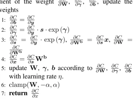
Algorithm 2The back-propagation of linear layer

Input: input x, weights W, γ andb, binarized

weightWb_{, temporary values(calculated in the}

propagation period), the gradient of the output∂C ∂y, learning rateη, binary weight rangeα

Output: the gradient of the input ∂C

∂x, the gra-dient of the weight ∂C

∂W, ∂C∂γ, ∂C∂b, update the weights

1: ∂C_∂b = ∂C_∂y

2: ∂C_∂γ = ∂C_{∂y ·}s_·exp (γ)

3: ∂C_∂s = ∂C_∂y ·exp (γ), _∂∂C_Wb = ∂C_∂sx, _∂∂C_W =

∂C ∂Wb

4: ∂C_∂x = ∂C_∂sWb

5: update W, γ, b according to ∂C

∂W, ∂C∂γ, ∂C∂b with learning rateη.

6: clamp(W,₋α, α)

7: return ∂C_∂x

The structure of the input embeddings and the output embeddings of the binarized LSTM lan-guage model is similar to the binarized embedding language model. The embeddings are binarized and additional linear layers are added after the in-put embedding layer and in front of the outin-put embedding layer. However, the additional linear layers are also binarized according to Algorithm1

and Algorithm2.

3.4 Memory Reduction

Denote the size of the vocabulary as V, and the size of the embedding and hidden layer asH. The memory consumptions of a one-layer LSTM lan-guage model, BELM and BLLM are listed in Ta-ble1.

Model Memory (bytes)

LSTM 8V H+ 32H2+ 16H BELM 0.25V H+ 40H2_{+ 24H}

BLLM 0.25V H+ 1.25H2_{+ 48H}

Table 1: Memory Requirements

For a language model, the vocabulary size is usually much larger than the hidden layer size. The main memory consumption comes from the embedding layers, which require 8V H bytes for an LSTM language model. Binarized embeddings can reduce this term to 0.25V H bytes. Further compression of the LSTM can drop the coefficient ofH2_{from32to1.25.}

4 Experiments

4.1 Experimental Setup

Our model is evaluated on the English Penn TreeBank (PTB) (Marcus et al., 1993), Chinese short message (SMS) and SWB-Fisher (SWB). The Penn TreeBank corpus is a famous English dataset, with a vocabulary size of 10K and 4.8% words out of vocabulary (OOV), which is widely used to evaluate the performance of a language model. The training set contains approximately 42K sentences with 887K words. The Chinese SMS corpus is collected from short messages. The corpus has a vocabulary size of about 40K. The training set contains 380K sentences with 1931K words. The SWB-Fisher corpus is an English corpus containing approximately 2.5M sentences with 24.9M words. The corpus has a vocabulary size of about 30K. hub5e is the dataset for the SWB ASR task.

human-assigned similarity judgments. The col-lection can be used to train and test computer al-gorithms implementing semantic similarity mea-sures. A combined set (combined) is provided that contains a list of all 353 words, along with their mean similarity scores. (Finkelstein et al.,

2001) The MEN dataset consists of 3,000 word pairs, randomly selected from words that occur at least 700 times in the freely available ukWaC and Wackypedia corpora combined (size: 1.9B and 820M tokens, respectively) and at least 50 times (as tags) in the open-sourced subset of the ESP game dataset. In order to avoid picking unrelated pairs only, the pairs are sampled so that they repre-sent a balanced range of relatedness levels accord-ing to a text-based semantic score (Bruni et al.,

2014).

First, we conduct experiments on the PTB, SWB and Text8 corpora respectively to evaluate language modeling performance. We use perplex-ity (PPL) as the metric to evaluate models of dif-ferent sizes. Then, the models are evaluated on ASR rescoring tasks. Rescoring the 100-best sen-tences generated by the weighted finite state trans-ducer (WFST), the model is evaluated by word er-ror rate (WER). Finally, we conduct experiments on word similarity tasks to evaluate whether the word embeddings produced by our models lose any information.

4.2 Experiments in Language Modeling

For traditional RNN based language models, the memory consumption mainly comes from the em-bedding layers (both input and output layers). However, when the hidden layer size grows, the memory consumption of the RNN module also be-comes larger. So the total memory usage relates to both the vocabulary size and hidden layer size, as mentioned in section3.4.

Experiments are conducted in language mod-eling to evaluate the model on the PTB, SWB, and SMS corpora respectively. In language mod-eling tasks, we regularize the networks using dropout(Zaremba et al., 2014). We use stochas-tic gradient descent (SGD) for optimization. The batch size is set to 64. For the PTB corpus, the dropout rate is tuned for different training settings. For the SWB corpus, we do not use dropout tech-nique. For the SMS corpus, the dropout rate is set to 0.25. We train models of different sizes on the three corpora and record the memory

us-age of the trained models. The initial learning rate is set to 1.0 for all settings. Since PTB is a rel-atively small dataset and the convergence rates of the BELM and the BLLM are slower than LSTM language model, we reduce the learning rate by half every three epochs if the perplexity on the validation set is not reduced. For the other experi-ments, the learning rate is always reduced by half every epoch if the perplexity on the validation set is not reduced. As introduced in section3, the bias of the output embedding layer is omitted. Adding bias term in the output embedding layer leads to small performance degradation in the BELM and the BLLM model, although it leads to a small im-provement in the LSTM model. This phenomenon may be related to optimization problems.

Hidden

size LSTM BELM BLLM Memory

PPL 500 48.0M91.8 11.3M88.0 1.6M95.2

Memory

PPL 1000 112.0M89.4 42.5M85.7 3.8M94.9

Table 2: Performances on the English PTB corpus

Hidden

size LSTM BELM BLLM Memory

PPL 500 129.1M57.6 13.8M58.4 4.1M60.4

Memory

PPL 1000 274.2M56.1

47.6M

55.6 8.9M56.2

Table 3: Performance on the English SWB corpus

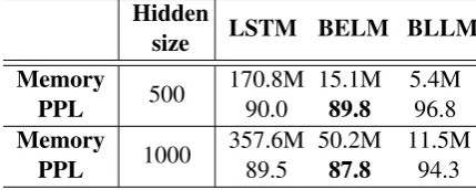
Hidden

size LSTM BELM BLLM Memory

PPL 500 170.8M90.0

15.1M

89.8 5.4M96.8

Memory

PPL 1000 357.6M89.5 50.2M87.8 11.5M94.3

Table 4: Performance on the Chinese SMS corpus

outperform the baseline LSTM LM. The small model (500 LSTM units) has a relative PPL im-provement of 4.1%and achieves a compression ra-tio of 4.3 and the large model (1000 LSTM units) also has a relative PPL improvement of 4.1%and achieves a compression ratio of 2.6. On the SWB corpus, the BELM models still perform well pared with the baseline model and achieve com-pression ratios of 9.4 and 5.8 respectively for the small and large models. On the SMS corpus, the BELMs model also gains relative PPL improve-ments of 0.2%and 1.9%, and achieves compres-sion ratios of 11.3 and 7.1 respectively. In sum-mary, the BELM model performs as well as the baseline model both on English and Chinese cor-pora, and reduces the memory consumption to a large extent.

The BLLM model, however, does not outper-form the baseline model, but still has acceptable results with a minor loss of performance. Since both the LSTM model and the embeddings are bi-narized, the total compression ratio is quite sig-nificant. The average compression ratio is about 32.0, so the memory consumption of the language model is significantly reduced.

We also study the performance of pruning the LSTM language model. We prune each parame-ter matrix and the embedding layers with various pruning rates respectively, and fine-tune the model with various dropout rates. In our experiments, pruning 75% parameter nodes hardly affects the performance. However, if we try pruning more parameter nodes, the perplexity increases rapidly. For example, for the English PTB dataset, when we prune95%parameter nodes of the embedding layers of an LSTM language model (500 LSTM units), the perpexity will increase from 91.8 to 112.3. When we prune 95% parameter nodes of an LSTM language model (500 LSTM units), the perplexity will increase from 91.8 to 132.3. There-fore, the effect of pruning is not as good as bina-rization for the language modeling task.

Binarization can be considered as a special case of quantization, which quantizes the parameters to pairs of opposite numbers. So, compared to nor-mal quantization, binarization can achieve a better compression ratio. In addition, for binarization, we do not need to determine the position of each unique values in advance. Therefore, binarization is more flexible than quantization.

We then study the effect of extra binary linear

layers in the BLLM. The additional binary linear layer after the input embedding layer and the ad-ditional binary linear layer in front of the output embedding layer are removed respectively in this experiment. We use well-trained embeddings to initialize the corresponding embedding layers and do the binarization using the method proposed in (Rastegari et al.,2016) when the additional binary linear layer is removed. The perplexities are listed in Table5. No-i means no additional binary linear layer after the input embedding layer. No-o means no additional binary linear layer in front of the out-put embedding layer. No-io means no additional binary linear layers. The experiment is conducted on the PTB corpus.

Hidden

size BLLMBLLMno-i BLLMno-o BLLMno-io PPL 500 95.2 95.2 101.7 100.3

PPL 1000 94.9 94.5 96.7 96.3

Table 5: Performances on the English PTB corpus

If the additional binary linear layer after the in-put embedding layer is removed, the performance does not drop, and even becomes better when the hidden layer size is1000. Although the additional binary layer after the input embedding layer is re-moved, the float version of the input embeddings of BLLM no-i is initialized with well-trained em-beddings, while the BLLM is not initialized with the well-trained embeddings. We think initializa-tion is the reason why the BLLM no-i performs comparatively to the BLLM. We also observe a PPL increase of 1-2 points for BLLM no-i if the input embeddings are not pre-trained (not listed in the table). This phenomenon prompts us to pre-train embeddings, which we leave to future work. Once the additional binary linear layer in front of the output embedding layer is removed, the perfor-mance degradation is serious. This shows that the output embeddings of the language model should not be directly binarized; the additional binary lin-ear layer should be inserted to enhance the model’s capacity, especially for low dimensional models.

4.3 Experiments on ASR Rescoring Tasks

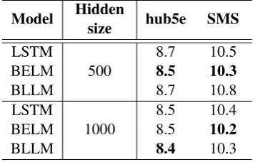
(very deep CNN) model on the 300-hour task is applied as the acoustic model. For the Chinese SMS dataset, the acoustic model is a CD-DNN-HMM model. The weighted finite state trans-ducer (WFST) is produced with a 4-gram language model. Then our language models are utilized to rescore the 100-best candidates. The models are evaluated by the metric of word error rate (WER).

Model Hidden_size hub5e SMS

LSTM 8.7 10.5

BELM 500 8.5 10.3

BLLM 8.7 10.8

LSTM 8.5 10.4

BELM 1000 8.5 10.2

BLLM 8.4 10.3

Table 6: Performances on ASR rescoring tasks

Table 6 shows the results on ASR rescoring tasks. The BELM model and BLLM model perform well both on the English and Chinese datasets. The BELM model achieves an absolute 0.2%WER improvement compared with the base-line model in three of the experiments. The BLLM model also has good results, even though it per-forms not so well in language modeling. The re-sults show that our language models work well on ASR rescoring tasks even with much less memory consumption.

4.4 Investigation of Binarized Embeddings

The experiments above show the good perfor-mances of our models. We also want to investigate whether the binarized embeddings lose any infor-mation. So, the embeddings are evaluated on two word similarity tasks. Experiments are conducted on the WS-353 and MEN tasks. We have trained the baseline LSTM model, the BELM model and BLLM model of a medium size on the Text8 cor-pus. We binarize the embeddings of the trained baseline LSTM model to investigate whether there is any loss of information by the simple binariza-tion method (labeled LSTM-bin in the table be-low). For each dimension, we calculate the mean and set the value to 1 if it is bigger than the mean, otherwise, we set it to -1.

The embedding size and the hidden layer size are set to 500. We use stochastic gradient descent (SGD) to optimize our models. We use cosine

dis-tance to evaluate the similarity of the word pairs. Spearman’s rank correlation coefficient is calcu-lated to evaluate the correlation between the two scores given by our models and domain experts.

Model PPL

LSTM 166.0

BELM 164.7

BLLM 172.3

Table 7: Language modeling performance on the Text8 corpus

Model WS-353 MEN

LSTM 53.1 46.3

LSTM-bin 25.5 19.4

BELM 49.1 47.0

BLLM 56.0 52.2

Table 8: Performances on the word similarity tasks

Table7shows our models perform well in lan-guage modeling on the Text8 corpus. Table 8

summarizes the performance of the word embed-dings in the similarity tasks. The embedembed-dings generated by the simple binarization method per-form obviously worse than the other embeddings, which indicates that much information is lost. The BELM model outperforms the baseline model on the MEN task, although it doesnt perform as well as the baseline model on the WS-353 task. How-ever, the MEN dataset contains many more word pairs, which makes the results on this dataset more convincing. The BLLM model significantly out-performs the baseline model on the two tasks. The results indicate that the binarized embeddings of the BLLM do not lose any semantic information although the parameters are represented only by -1 and 1.

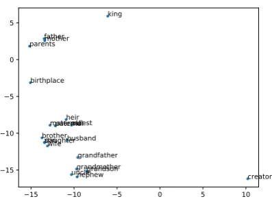
We suspect that binarization plays a role in reg-ularization and produces more robust vectors. We also give an example visualization of some word vectors. The dimension of the embeddings of the BLLM is reduced by TSNE (Maaten and Hinton,

2008). The words which are the closest tofather

(according to the cosine distance of word vectors) are shown in Figure1.

In this figure,motherandparentsare the clos-est words to father, which is quite understand-able. The words husband, wife, grandfather

indicat-−15 −10 −5 0 5 10 −15

−10 −5 0 5

father mother

son eldest parents

uncle grandfather wife husband daughter

maternal

creator paternal

brother

grandson heir

nephew grandmother

king

birthplace

Figure 1: Visualization of the Binarized Embeddings

ing the embeddings indeed carry semantic infor-mation.

5 Conclusion

In this paper, a novel language model, the bina-rized embedding language model (BELM) is pro-posed to solve the problem that NN based lan-guage models occupy tremendous space. For tra-ditional RNN based language models, the memory consumption mainly comes from the embedding layers (both input and output layers). However, when the hidden layer size grows, the memory consumption of the RNN module also becomes larger. So, the total memory usage relates to both the vocabulary size and hidden layer size. In the BELM model, words are represented in the form of binarized vectors, which only contain parame-ters of -1 or 1. For further compression, we bina-rize the long short-term memory language model combined with the binarized embeddings. Thus, the total memory usage can be significantly re-duced. Experiments are conducted on language modeling and ASR rescoring tasks on various cor-pora. The results show that the BELM model per-forms well without any loss of performances at compression ratios of 2.6 to 11.3, depending on the hidden and vocabulary size. The BLLM model compresses the model parameters almost thirty-two times with a slight loss of performance. We also evaluate the embeddings on word similarity tasks. The results show the binarized embeddings even perform much better than the baseline em-beddings.

6 Future Work

In the future, we will study how to improve the performance of the BLLM model. And, we will research methods to accelerate the training and re-duce the memory consumption during training.

Acknowledgments

The corresponding author is Kai Yu. This work has been supported by the National Key Re-search and Development Program of China under Grant No.2017YFB1002102, and the China NSFC projects (No. 61573241). Experiments have been carried out on the PI supercomputer at Shanghai Jiao Tong University.

References

Yoshua Bengio, R´ejean Ducharme, Pascal Vincent, and Christian Jauvin. 2003. A neural probabilistic lan-guage model.Journal of machine learning research

3(Feb):1137–1155.

Elia Bruni, Nam-Khanh Tran, and Marco Baroni. 2014. Multimodal distributional semantics. J. Artif. Intell. Res.(JAIR)49(2014):1–47.

Di Cao and Kai Yu. 2017. Deep attentive structured language model based on lstm. In International Conference on Intelligent Science and Big Data En-gineering. Springer, pages 169–180.

Junyoung Chung, Caglar Gulcehre, KyungHyun Cho, and Yoshua Bengio. 2014. Empirical evaluation of gated recurrent neural networks on sequence model-ing.arXiv preprint arXiv:1412.3555.

Matthieu Courbariaux, Yoshua Bengio, and Jean-Pierre David. 2015. Binaryconnect: Training deep neural networks with binary weights during propagations. InAdvances in Neural Information Processing Sys-tems. pages 3123–3131.

Matthieu Courbariaux, Itay Hubara, Daniel Soudry, Ran El-Yaniv, and Yoshua Bengio. 2016. Bina-rized neural networks: Training deep neural net-works with weights and activations constrained to+ 1 or-1.arXiv preprint arXiv:1602.02830.

Marcus Edel and Enrico K¨oppe. 2016. Binarized-blstm-rnn based human activity recognition. In

Indoor Positioning and Indoor Navigation (IPIN), 2016 International Conference on. IEEE, pages 1– 7.

Song Han, Huizi Mao, and William J Dally. 2015. Deep compression: Compressing deep neural net-works with pruning, trained quantization and huff-man coding. arXiv preprint arXiv:1510.00149.

Sepp Hochreiter and J¨urgen Schmidhuber. 1997. Long short-term memory. Neural computation

9(8):1735–1780.

Lu Hou, Quanming Yao, and James T Kwok. 2016. Loss-aware binarization of deep networks. arXiv preprint arXiv:1611.01600.

Itay Hubara, Matthieu Courbariaux, Daniel Soudry, Ran El-Yaniv, and Yoshua Bengio. 2016. Binarized neural networks. InAdvances in neural information processing systems. pages 4107–4115.

Sergey Ioffe and Christian Szegedy. 2015. Batch nor-malization: Accelerating deep network training by reducing internal covariate shift. In International Conference on Machine Learning. pages 448–456.

Laurens van der Maaten and Geoffrey Hinton. 2008. Visualizing data using t-sne. Journal of Machine Learning Research9(Nov):2579–2605.

Mitchell P. Marcus, Mary Ann Marcinkiewicz, and Beatrice Santorini. 1993. Building a large anno-tated corpus of English: the penn treebank. MIT Press.

Tomas Mikolov, Martin Karafit, Lukas Burget, Jan Cernock, and Sanjeev Khudanpur. 2010. Recur-rent neural network based language model. In IN-TERSPEECH 2010, Conference of the International Speech Communication Association, Makuhari, Chiba, Japan, September. pages 1045–1048.

Yanmin Qian, Mengxiao Bi, Tian Tan, Kai Yu, Yan-min Qian, Mengxiao Bi, Tian Tan, and Kai Yu. 2016. Very deep convolutional neural networks for noise robust speech recognition. IEEE/ACM Trans-actions on Audio Speech & Language Processing

24(12):2263–2276.

Mohammad Rastegari, Vicente Ordonez, Joseph Red-mon, and Ali Farhadi. 2016. Xnor-net: Imagenet classification using binary convolutional neural net-works. In European Conference on Computer Vi-sion. Springer, pages 525–542.

Xu Xiang, Yanmin Qian, and Kai Yu. 2017. Binary deep neural networks for speech recognition. Proc. Interspeech 2017pages 533–537.

Wojciech Zaremba, Ilya Sutskever, and Oriol Vinyals. 2014. Recurrent neural network regularization.