Proceedings of NAACL-HLT 2018, pages 1605–1614
Combining Deep Learning and Topic Modeling for Review Understanding
in Context-Aware Recommendation
Mingmin Jin1 Xin Luo1 Huiling Zhu1,2 Hankz Hankui Zhuo1,2∗ 1School of Data and Computer Science, Sun Yat-Sen University 2Guangdong Key Laboratory of Big Data Analysis and Processing
Guangzhou, China
{jinmm1,luox351,zhuhling62,zhuohank2}@{mail21,mail2}.sysu.edu.cn
Abstract
With the rise of e-commerce, people are ac-customed to writing their reviews after receiv-ing the goods. These comments are so impor-tant that a bad review can have a direct impact on others buying. Besides, the abundant in-formation within user reviews is very useful for extracting user preferences and item prop-erties. In this paper, we investigate the ap-proach to effectively utilize review informa-tion for recommender systems. The proposed model is named LSTM-Topic matrix factor-ization (LTMF) which integrates both LSTM and Topic Modeling for review understand-ing. In the experiments on popular review dataset Amazon , our LTMF model outper-forms previous proposed HFT model and Con-vMF model in rating prediction. Furthermore, LTMF shows the better ability on making topic clustering than traditional topic model based method, which implies integrating the infor-mation from deep learning and topic modeling is a meaningful approach to make a better un-derstanding of reviews.
1 Introduction
Recommender systems (RSs) are widely used in the field of electronic commerce to provide per-sonalized recommendation services for customers. Most popular RSs are based onCollaborative Fil-tering (CF), which makes use of users’ explicit ratings or implicit behaviour for recommendations (Koren, 2008). But CF models suffer from data sparsity, which is also called “cold-start” prob-lem. Models perform poorly when there is few available data. To alleviate this problem, utiliz-ing user reviews can be a good approach because user reviews can directly reflect users’ preferences and items’ properties and exactly correspond to the user latent factors and item latent factors in CF models.
∗
corresponding author
To understand user reviews, previous ap-proaches are mainly based on topic modeling, a suite of algorithms that aim to discover the the-matic information among documents (Blei,2012). The simplest and commonly used topic model is latent dirichlet allocation(LDA). Recently, as deep learning shows great performance in com-puter vision (Krizhevsky et al., 2017) and NLP (Kim, 2014), some approaches combining deep learning with CF are proposed to capture latent context features from reviews.
However, we find there are some limitations in existing models. First, the LDA algorithm used in previous models like Hidden Factors as Top-ics (HFT) (McAuley and Leskovec,2013) ignores contextual information. If a user writes “I pre-fer apple than banana when choosing fruits” in a review, we can clearly know the user’s prefer-ence and recommend items including apple. But LDA ignores the structural information and con-siders the two words as the same since they both appear once in the sentence.
Compared with topic modeling, deep learning methods such as Convolutional Neural Network (CNN) andRecurrent Neural Network(RNN) are able to retain more context information. CNN uses sliding windows to capture local context and word order. RNN considers a sentence as a word se-quence, and the former word information will be reserved and passed back, which gives RNN the ability to retain the whole sentence information.
But these still exist some problems. For CNN, the sizes of sliding windows are often small, which causes CNN model fails to link words in the sen-tence begin and end. Given the review “I prefer apple than google when choosing jobs”, CNN can not notice the two words ’apple’ and ’jobs’ simultaneously if the windows size is small, so it will meet the ambiguity problem that the word ’apple’ means fruit or company. For RNN,
though it performs better than CNN on persisting former information, the information will still de-creases with the length of sentences increasing. So when a review is long, the effect of RNN is lim-ited.
Faced with these problems, we propose to inte-grate deep learning and topic modeling to extract more global context information and get a deeper understanding of user reviews. Deep learning methods can reserve context information, while topic modeling can provide word co-occurrence relation to make a supplement for information loss.
We useLong Short-Term Memory(LSTM) net-work for the deep learning part, because it is a special type of RNN which has better perfor-mance on gradient vanishing and long term depen-dence problems than vanilla RNN structure. We use LDA for the topic modeling part. Then the two parts are integrated into a matrix factoriza-tion framework. The final model is named LSTM-Topic matrix factorization(LTMF).
Furthermore, as the topic modeling part and deep learning part are connected in our model, the topic clustering results will be influenced by the deep learning information. In experiments, LTMF shows a better topic clustering ability than tradi-tional LDA based HFT model. This gives us some inspiration on using the integrating methods into other tasks like sentiment classification.
In the remainder of the paper, we first review previous work related to our work. Then we address preliminaries and present our models in detail. After that we evaluate our approach by comparing our approach with state-of-the-art algo-rithms. Finally we conclude the paper with future work.
2 Related Work
There has been some earlier approaches to ex-tract review information for RSs. Wang and Blei
(2011) proposed collaborative topic regression (CTR) that combined topic modeling and collabo-rative filtering in a probabilistic model. McAuley and Leskovec(2013) developed a statistical model HFT using a transfer function to combine rating and review tightly.Ling et al.(2014) andBao et al.
(2014) proposed models similar to CTR and HFT with some structural differences.
Recently, several researchers begin to utilize deep learning in RSs. Wang et al. (2015)
pre-sented a Bayesian modelcollaborative deep learn-ing (CDL) leveraging SDAE neural networks as a text feature learning component. Bansal et al.
(2016) trained agated recurrent units(GRUs) net-work to encode text sequences into latent vectors.
Zhao et al.(2016) trained a deep CNN to discover the abstract representation of movie posters and still frames, and incorporated it into a neighbor-hood CF model. Kim et al. (2016) utilized CNN to retain contextual information in review, and de-veloped a document context-aware recommenda-tion model (ConvMF). The ConvMF model is a re-cently proposed model and is shown to outperform PMF and CDL, and we choose it as a baseline in our experiments.Zheng et al.(2017) proposed the Deep Cooperative Neural Networks(DeepCoNN) model which constructed two concurrent CNN to simultaneously model user and item reviews and then combined the features into Factorization Ma-chine. Attention in neural networks has been pop-ular in nearly years,Seo et al.(2017) proposed a model using CNN with dual attention for rating prediction. There are some similarity between the D-attn model with our LTMF model for we both want to extract more global information, where they use attention CNN model and we utilize the information from both topic modeling and deep learning. The D-attn model fail to work if there is not enough reviews, while our LTMF model use review information as a supplementary of rating. So it can still work effectively even there are few reviews.
Besides, Diao et al.(2014) proposed a method jointly modeling aspects, sentiments and ratings for movie recommendation. Hu et al.(2015) pro-posed MR3 model to combine ratings, social re-lations and reviews together for rating prediction. These hybrid models boost the performance than individual components, which also give us some inspiration on proposing the LTMF framework.
3 Preliminary
3.1 Notations
We use explicit ratings as the training and test data. Suppose there areM users
U ={u1, u2, ..., ui, ..., uM}
andN items
where each user and item is represented by aK -dimension latent vector, ui ∈ RK and vj ∈
RK. The rating sparse matrix is denoted asR ∈
RM×N, wherer
ij is the rating of userui on item
vj. Dis the review (document) corpus wheredij
is the review of useruion itemvj.
3.2 PMF: a standard matrix factorization model
Probabilistic Matrix Factorization (PMF) (Mnih and Salakhutdinov, 2008) is an effective recom-mendation model that uses matrix factorization (MF) technique to find the latent features of users and items from a probabilistic perspective. In PMF, the predicted ratingRˆij is expressed as the
inner product of user latent vectoruiand item
la-tent vectorvj :Rˆij =uTi vj. To get latent vectors,
PMF minimises the following loss function:
L= M
X
i N
X
j
Iij(Rij −uTi vj)2
+λu M
X
i
kuik2F +λv N
X
j
kvj k2F, (1)
where Rij is the observed rating. The first part
of Eq.(1) is the sum-of-squared-error between pre-dicted and observed ratings and the second part is quadratic regularization terms to avoid over-fitting. λu and λv are corresponding
regulariza-tion parameters.Iijis the indicator function which
equals 1 ifi-th user ratedj-th item, and equals 0 otherwise.
3.3 HFT: understand reviews through topic modeling
Hidden Factors as Topics (HFT) (McAuley and Leskovec, 2013) provides an effective approach to integrates topic modeling into traditional CF models. It utilizes LDA, the simplest topic model which assumes there are k topics T =
{t1, t2, ..., tk} in document corpus D. Each
doc-ument d ∈ Dhas a topic distribution θd overT
and each topic has a word distribution φ over a fixed vocabulary. To connect the document-topic distributionθand item factorsv, HFT proposes a transformation function:
θj,k =
exp(κvj,k)
P
kexp(κvj,k)
, (2)
wherevj,k is the k-th latent factor in item vector
vj and θj,k is the k-th topic probability in item
document-topic distributionθj,κis the parameter
controlling the “peakiness” of the transformation.
Besides, HFT introduces an additional variableψ to ensure the word distributionφk is a stochastic
vector which satisfiesPwφk,w = 1, the relation
is denoted as follows: φk,w=
exp(ψk,w)
P
wexp(ψk,w)
s.t. X
w
φk,w= 1.
(3) The final loss function is :
L= M
X
i N
X
j
Iij(Rij−Rˆij)2
−λt N
X
d
X
n∈Nd
logθd,zd,nφzd,n,wd,n, (4)
where Rˆij is predicted ratings, θ and φ are the
topic and word distribution respectively, wd,n is
then-th word in documentdandzd,nis the word’s
corresponding topic,λtis a regularization
param-eters.
4 The LTMF Model
We propose the LSTM-Topic matrix factorization (LTMF) model, which integrates LSTM and topic modeling for recommendation. The model utilizes both rating and review information. For the rating part, we use probabilistic matrix factorization to extract rating latent vectors. For the review part, we use LDA (following the way of HFT) to extract topic latent vectors and adopt an LSTM architec-ture to generate document latent vectors . Then we combine the three vectors into a unified model. The overview of LTMF model is shown in Figure
1.
4.1 Parameter Relation
The left of Figure 1 is the parameters relations in LTMF model, which can be divided into three parts: Θ = {U,V}is the parameters associated with rating MF,Φ ={θ, φ}is the parameters asso-ciated with topic model,Ω ={W, l}is the param-eters associated with LSTM. The shaded nodes are data (R:rating, D: reviews) where the others are parameters. Single connection lines represent there are constraint relationship between the two nodes. Double connections (e.g. V andθ) mean the relationship is bidirectional so they can affect each other’s results.
4.2 LSTM Architecture
se-φ
R D
l
Wu
v
θ
Topic Modeling
LSTM PMF
Document sequence:Dj
Embedding layer
LSTM LSTM
prefer when choosing fruits
LSTM
apple than banana
LSTM LSTM LSTM LSTM LSTM LSTM layer
I
Full Connect layer
LSTM latent vector
Document latent vector:lj
...
p p p p
...
[image:4.595.74.524.62.234.2]LSTM Structure
Figure 1: The overview of LTMF model. Left:Parameters relations of LTMF. Right:the detailed LSTM architec-ture.
quenceDj. Every word in the document sequence
Dj = (w1, w2, ..., wnj) will firstly be embedded
into apdimension vector. Next, word vectors are sent into LSTM network according to the word or-der inDj and produces a latent vector. Finally, the
latent vector is sent to a full connect layer whose output is the document latent vectorlj. The above
process can be written as:
lj =LST M(Dj, W), (5)
whereDj is the input document sequence,W
rep-resents weights and bias variables in LSTM net-work.
4.3 Probabilistic Prior
Gaussian distribution is the basic prior hypothe-sis in our model. We place zero-mean spherical Gaussian priors on user latent features u, LSTM weightsW and observed ratingsR. For item vec-torv, we place the Gaussian prior on its difference with LSTM outputlj:
p(v|lj, σv2) = N
Y
j=1
N(vj−lj|0, σv2I)
= N
Y
j=1
N(vj|lj, σv2I).
The function is important for connecting rat-ings and reviews. Although document vector lj
is closed to item feature vectorvj for they both
re-flect item’s properties. There still exists some dis-crepancies. For example, when writing reviews, users usually write more about appearance and only briefly mention price. So in review based document vector lj, the weight of “appearance”
will be larger than rating based latent vector vj.
To preserve the discrepancy between vj and lj ,
we import the Gaussian noise vectorσvas the
off-set.
4.4 Objective Function
Finally, we maximize the log-posterior of the three parts and get the objective function as follows:
L= M
X
i N
X
j
Iij(Rij −uTi vj)2
−λt N
X
d
X
n∈Nd
logθzd,nφzd,n,wd,n
+λu M
X
i
kuik2F +λv N
X
j
kvj−lj k2F
+λW Nk
X
k
kWkk2F, (6)
whereNkis the number of weighs in LSTM
net-work,λu, λv, λW are regularization parameters.z
is the topic assignment for each word,λtis the
reg-ularization parameters to control the proportion of topic part.
The objective function of LTMF can be con-sidered as an extended PMF model where the formation from topic modeling and LSTM is in-cluded as regular terms. In the next section, we will explain how LTMF leverages the information from topic modeling and LSTM, and why LTMF can combine the information of the two parts.
4.5 The Effectiveness of LTMF
result of item vectors. If we take partial derivative of Eq.(6) with respect to vj, the constraint
rela-tionship can be clearer: ∂L
∂vj =
M
X
i=1
2Iij(Rij−uTi vj)ui+ 2λv(vj −lj)
−λtκ K
X
k=1
(nj,k−Nj
exp(κvj,k)
P
exp(κvj,k)
), (7)
In Eq.(7), the optimization direction of vj is
subject to two regular terms. The former one is controlled by LSTM vector lj. The latter one
is controlled by topic parameters (κ, nj,k, Nj).
Hence, we can leverages the information from both LSTM and topic modeling for recommenda-tion.
Besides, note the double connections between item vector V and topic distribution θ in Figure
1. They mean the information from topic model-ing can affect the result ofV, while the change in V can also be passed to topic part and affect the review understanding result of topic modeling by Eq.2. For V and LSTM vectorl, the analysis is the same. Indeed, item vectorsV plays the role of transporter to connect LSTM part and topic mod-eling part. This is why LTMF can combine the information of topic modeling and LSTM to make a deeper understanding of user reviews.
Furthermore, LTMF provides an effective framework to integrate topic model with deep learning networks for recommendation. In ex-periments, we replace the LSTM part with CNN to make a comparison model. Experiments show both models boost the rating prediction accuracy.
4.6 Optimization
Our objective is to search:
arg min
Θ,Φ,z,κ,ΩL
(Θ,Φ, z, κ,Ω). (8)
Recall thatΘis the parameters associated with rat-ings MF,Φis the parameters associated with topic
modeling,zis the topic assignment for each word, κ is the peakiness parameter to control the trans-formation between item vector v and topic dis-tribution θ, Ω is the parameters associated with
LSTM.
For vj is coupled with the parameters of topic
modeling and LSTM vector, we cannot optimize these parameters independently. We adopt a pro-cedure that alternates between two steps. In each step we fix some parameters and optimize the oth-ers. The optimization process is shown below:
1. solve the objective by fixingztandΩt: arg min
Θ,Φ,κL(Θ,Φ, z
t, κ,Ωt)
to updateΘt+1,Φt+1,κt+1.
2. (a) updateΩt+1 with fixingvjt+1 and
doc-ument sequenceDj.
(b) samplezd,jt+1with probability p(zd,jt+1 =k) =φtk,wd,j+1 .
In the step 1, we fixzandΩto update remaining
termsΘ,Φ, κby L-BFGS algorithm. In the step 2, we fixΘ,Φandκto update LSTM parametersΩ
and topic model parametersz. Since LSTM part and topic part are independent when item vectors V are certain, we can update the two term respec-tively. In step 2(a), we update Ωby back
prop-agation algorithm. With fixing the other parame-ters, the objective function of W can be seen as a weighted squared error function (k vj−lj k2F)
withL2regularized terms (kW k2F), which means
we can useDjas the input andvjis the label to run
the back propagation process. In step 2(b), we iter-ates through all documents and each word within to update zd,j via Gibbs Sampling. The reason
why we do not divide the process into three steps is that the step 2(a) and 2(b) are independent with step 1 finished, which means we can parallelize the two steps.
Finally, we repeat these two steps until conver-gence. In practice, we run the step 1 with 5 gra-dient iterations using LBFGS, then we iterate the LSTM part 5 times. At the same time, we update the topic model part once. The whole process is called a cycle, and it usually takes 30 cycles to reach a local optimum.
In addition to the gradient of vj, the gradients
of other parameters used in step 1 are listed as fol-lows:
∂L ∂ui
= N
X
j=1
2Iij(Rij−uTi vj)vj+ 2λuui. (9)
∂L
∂ψ =−λt
Nw
X
w=1 K
X
k=1
nk,w−Nk
exp(ψk,w)
zw
(10)
∂L
∂κ =−λt
N
X
j=1 K
X
k=1 vj,k
njk−Nj
exp(κvj,k)
zj
.
Dataset users items ratings av. words per item density Amazon Instant Video (AIV) 29753 15147 135167 86.69 0.0030%
[image:6.595.87.515.61.222.2]Apps for Android (AFA) 240931 51599 1322839 65.80 0.0106% Baby (BB) 71812 42515 379969 81.83 0.0124% Musical Instruments (MI) 29005 48751 150526 86.44 0.0106% Office Product (OP) 59844 60628 286521 82.41 0.0079% Pet Supplies (PS) 93270 70063 477859 78.86 0.0073% Grocery Gourmet Food (GGF) 86389 108448 508676 76.97 0.0054% Video Games (VG) 84257 39422 476546 92.55 0.0143% Patio Lawn and Garden (PLG) 54167 57826 242944 82.22 0.0078% Digital Music (DM) 56812 156496 351769 38.79 0.0040%
Table 1: Statistics of datasets.
w occurs in topic k; Nw is the word vocabulary
size of the document corpus;Nk is the number of
words in topick;nj,kis the number of times when
topickoccurs in the document of itemj;Njis the
total number of words in document j; zw andzj
are the corresponding normalizers:
zw = K
X
k=1
exp(ψk,w), zj = K
X
k=1
exp(κvj,k).
5 Experiment
5.1 Datasets
We use the real-world Amazon dataset1(collected
by McAuley et al. (2015)) for our experiments. For the original dataset is too large, we choose 10 sub datasets in experiments. To increase data density, we remove users which have less than 3 ratings. For raw review texts, we adopt the same preprocessing methods as ConvMF2: set the
max-imum length of a item document to 300; remove common stop words and document specific words which have document frequency higher than 0.5; choose top 8000 distinct words as the vocabulary; remove all non-vocabulary words to construct in-put document sequences. After preprocessing, the statistics of datasets are listed in Table 1, where the abbreviations of datasets are shown in paren-theses.
5.2 Evaluation Procedure 5.2.1 Baseline
The baselines used in our experiments are listed as follows:
1http://jmcauley.ucsd.edu/data/amazon/ 2http://dm.postech.ac.kr/ cartopy/ConvMF/
• PMF: Probabilistic Matrix Factorization (PMF) (Mnih and Salakhutdinov,2008) is a standard matrix factorization model for RSs. It only uses rating information.
• HFT: This is a state-of-art method that com-bines reviews with ratings (McAuley and Leskovec,2013). It utilizes LDA to capture unstructured textual information in reviews.
• ConvMF: Convolutional Matrix Factoriza-tion (ConvMF) (Kim et al., 2016) is a re-cently proposed recommendation model. It utilizes CNN to capture contextual informa-tion of item reviews.
• LMF: LSTM Matrix Factorization (LMF) is a submodel of LTMF without the topic part. We can compare it with ConvMF to show the effectiveness of LSTM than CNN on review understanding.
• CTMF: We modify the LTMF model by re-placing the LSTM part with CNN (following the structure of ConvMF) and construct the comparison model CNN-Topic Matrix Fac-torization (CTMF). CTMF can be used to evaluate the effectiveness of combining deep learning and topic modeling.
(a) (b) (c) (d) (e) (f)
Dataset PMF HFT ConvMF CTMF LMF LTMF
[image:7.595.306.527.284.466.2]AIV 1.436 (0.02) 1.368 (0.02) 1.388 (0.02) 1.350 (0.03) 1.321 (0.02) 1.309(0.02) AFA 1.673 (0.01) 1.649 (0.01) 1.651 (0.01) 1.648 (0.01) 1.635 (0.01) 1.629(0.01) BB 1.643 (0.01) 1.577 (0.01) 1.556 (0.02) 1.531 (0.01) 1.513 (0.02) 1.499(0.01) MI 1.555 (0.03) 1.423 (0.02) 1.399 (0.02) 1.367 (0.02) 1.317 (0.02) 1.302(0.02) OP 1.622 (0.02) 1.547 (0.02) 1.501 (0.02) 1.466 (0.02) 1.432 (0.02) 1.420(0.02) PS 1.796 (0.01) 1.736 (0.01) 1.698 (0.02) 1.680 (0.02) 1.646 (0.02) 1.626(0.01) GGF 1.585 (0.01) 1.539 (0.01) 1.478 (0.01) 1.446 (0.02) 1.393 (0.01) 1.386(0.01) VG 1.510 (0.02) 1.468 (0.01) 1.463 (0.01) 1.448 (0.01) 1.423 (0.01) 1.409(0.01) PLG 1.854 (0.02) 1.779 (0.02) 1.710 (0.02) 1.678 (0.02) 1.628 (0.02) 1.608(0.02) DM 1.197 (0.01) 1.171 (0.01) 1.032 (0.01) 0.990 (0.01) 0.968 (0.01) 0.965(0.01)
Table 2: MSE results of various models (K=5). The best results are highlighted in bold. The standard deviations of MSE results are shown in parenthesis.
5.2.2 Implementation Details
For all models, we set the dimension of user and item latent vectorsK = 5, and initialize the
vec-tors randomly between 0 and 1. Topic number and the dimension of document latent vectorlare also set to 5. For methods using deep learning, we initialized word latent vectors randomly with the embedding dimension p = 200. The
opti-mization algorithm used in back propagation is rmspropand the activation function used in fully connected layer istanh. In LSTM network, we set the output dimension to 128 and dropout rate 0.2. For CTMF, we adopt the same setting as ConvMF where the sliding window sizes is{3,4,5}and the shared weights per window size is 100.
Hyper parameters are set as follows. For PMF, λu = λv = 0.1. For HFT, we select λt ∈
{1,5} which gives better result in each experi-ment. For LMF and ConvMF, we set λu = 0.1
and λv = 5. For LTMF and CTMF, we select
λt∈ {0.05,0.1,0.5}which gives the lowest
vali-dation set error.
5.3 Quantitative analysis of rating prediction
We evaluate these models and report the lowest test set error on each dataset. The MSE results are shown in Table2where the best result of each dataset is highlighted in bold and the standard de-viations of corresponding MSE are recorded in parenthesis.
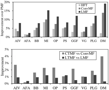
We can see that theLTMF model consistently outperform these baselines on all datasets. This clearly confirms the effectiveness of our proposed method. To make a more intuitive comparison, the improvement histograms of these models are
0% 5% 10% 15% 20%
AIV AFA BB MI OP PS GGF VG PLG DM
Impro
vement over PMF
HFT ConvMF LMF
0% 1% 2% 3% 4% 5%
AIV AFA BB MI OP PS GGF VG PLG DM
Improvmen
t CTMF vs ConvMFLTMF vs LMF
Figure 2: Above: Improvements of HFT, ConvMF and LMF, compared with PMF on different datasets. Be-low: Improvements of CTMF and LTMF, compared with ConvMF and LMF respectively.
shown in Figure2.
re-1.20 1.30 1.40 1.50 1.60 1.70 1.80 1.90 2.00
1 2 3 4 5 6 7 8 9 10
M
SE
a PMF b HFT c ConvMF d CTMF e LMF f LTMF
0.00 0.02 0.04 0.06 0.08 0.10 0.12 0.14 0.16
1 2 3 4 5 6 7 8 9 10
In
creas
ed
v
al
u
e
th
an
PMF
[image:8.595.75.525.64.178.2]HFT ConvMF CTMF LMF LTMF
Figure 3: Results for recommendation within limited ratings and reviews. Left: the MSE values of all models. Right: the incerase compared with PMF.
views understanding. As mentioned in Section 1, Topic Modeling based HFT only considers the co-existence of words in texts and ignores structural context information. CNN based ConvMF lacks the ability to capture global context information due to the size limitation of sliding windows. This is exactly what LSTM possesses and why LSTM based LMF model outperforms ConvMF.
The figure below is the comparison of two in-tegrated models (LTMF and CTMF) that import topic information with two original models that only use deep learning (LMF and ConvMF). We can see that both integrated models outperform the original models, which confirms our conjecture that recommendation results can be improved by combining structural and unstructured in-formation. For CTMF model, it makes over 2% improvement on 5 out of 10 datasets compared with ConvMF. As to LTMF model, it achieves nearly 1% improvements that LMF on 7 out of 10 datasets.
The reason why LTMF gains less promotion can be explained from two sides. Numerically, for the comparison model LMF is already a strong base-line proposed by ourselves, it’s more difficult to make a significant improvement. Theoretically, since LSTM can persist enough global informa-tion when the input sentence is relatively short, the supplements of topic information in LTMF are not so remarkable. As an illustration, we can com-pare the results on datasets “DM” and “VG”. For the dataset “DM”, as shown in Table1, it has the fewest words per item (38.79) and the improve-ment of LTMF is minimum. But for the dataset “VG”, it has the most words per item (92.55). The global context information obtained by LSTM will still decrease with such long sentences, and the topic information can make an effective supple-ment. So the improvement of LTMF on “VG” is
greater and comparable with CTMF.
5.4 Recommendation with different data sparsity
Rating data and review data are always sparse in RSs. To compare these models on making rec-ommendation in different data sparsity, especially for new users who only have limited ratings, we choose the dataset “Baby” and refilter it to make sure every user has at least N ratings (N varies from 1 to 10). A greater N means the user has rated more items, so the data sparsity problem is weaker. We test all models on the 10 subsets of “Baby” with the same dataset split ratio and text preprocessing. The final results are shown in Fig-ure3, where the left one is the MSE values of all models, and the right one is the increase of the other models compared with PMF.
We can observe that all models gain better rec-ommendation accuracy with the increment of user rating numberN. In other words, user and item latent features can be better extracted with more useful information. WhenN is small, especially whenN = {2,3}, the models which utilize both review and rating information achieve biggest im-provements over PMF. It suggests that review information can provide effective supplement when rating data is scarce. With the increase ofN, the improvements of all review used mod-els become smaller. This is because modmod-els can extract more features from gradually dense ratings data, and the effectiveness of review data begins to decrease. Same as the previous experiment, our LTMF model achieve the best results in the com-parison with other models.
5.5 Qualitative Analysis
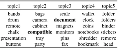
Office Product (OP)
topic1 topic2 topic3 topic4 topic5 envelope markers pins wallet planner
erasers compatible scale notebooks keyboard needs lead huge window tab numbers mail credit notebook remove
[image:9.595.80.283.66.157.2]letters nice documentcardboard stickers christmas camera attach plug clips
Table 3: Top topic words discovered by HFT
Office Product (OP)
[image:9.595.80.284.201.284.2]topic1 topic2 topic3 topic4 topic5 bands bags scale wallet folder drum camera document clock folders remote cabinet magnets coins binder chalk compatible monitors notebooks stickers presentation tray pins shredder remove buttons party fax bookmark head Table 4: Top topic words discovered by LTMF
proposed LTMF framework, the information ex-tracted by LSTM and Topic Modeling will both affect the final word clustering results. So, we can compare the topic words discovered by HFT and LTMF to evaluate whether combing LSTM and Topic Modeling is able to make a better un-derstanding of user reviews.
We choose the dataset “Office Product” (OP) and show the top topic words of HFT and LTMF in Table3and Table4. As we can see, there are many words existed in both tables (e.g. “wallet”, “note-books”, “document”). These words are closely re-lated to the category of dataset “Office Product”, which implies both models can get a good inter-pretation of user reviews.
However, when we carefully compare the two tables, there exists some differences. In Table3, there are some adjectives and verbs which have little help for topic clustering (e.g. “nice”, “huge”, “attach”), but they still get large weights and ap-pear in the front of topic words list. Obviously, HFT misinterprets these words for they usually appear together with the real topic words. In Ta-ble 4, we are not able to find them in top words list, because extra information from LSTM makes a timely supplement. Besides, similar situations also occur on words “document” and “compati-ble”. The word “document” is an apparent topic word, so LTMF gives it a larger weight in topic words list. For the word “compatible”, as an adjectives, it can provide less topic information than nouns, so LTMF decreases its weight and put
“camera” in the second place. From the above analysis we can see LTMF shows the better topic clustering ability than HFT.
6 Conclusion and Future Work
In this paper, we investigate the approach to ef-fectively utilize review information for RSs. We propose the LTMF model which integrates both LSTM and Topic modeling in context aware rec-ommendation. In the experiments, our LTMF model outperforms HFT and ConvMF in rating prediction especially when the data is sparse. Fur-thermore, LTMF shows better ability on making topic clustering than traditional topic model based method HFT, which implies integrating the infor-mation from deep learning and topic modeling is a meaningful approach to make a better understand-ing of reviews. In the future, we plan to evaluate more complex networks for recommendation tasks under the framework proposed by LTMF. Besides, we are interested to apply the method of comb-ing topic model and deep learncomb-ing into some tradi-tional NLP tasks.
Acknowledgments
We thank the National Key Research and Devel-opment Program of China (2016YFB0201900), National Natural Science Foundation of China (U1611262), Guangdong Natural Science Funds for Distinguished Young Scholar (2017A030306028), Pearl River Science and Technology New Star of Guangzhou, and Guang-dong Province Key Laboratory of Big Data Analysis and Processing for the support of this research.
References
Trapit Bansal, David Belanger, and Andrew Mc-Callum. 2016. Ask the gru: Multi-task learn-ing for deep text recommendations. In Proceed-ings of the 10th ACM Conference on Recommender Systems. ACM, New York, NY, USA, RecSys ’16, pages 107–114. https://doi.org/10.
1145/2959100.2959180.
Yang Bao, Hui Fang, and Jie Zhang. 2014. Top-icmf: Simultaneously exploiting ratings and re-views for recommendation. In Proceedings of the Twenty-Eighth AAAI Conference on Artificial Intelligence. AAAI Press, AAAI’14, pages 2–
8. http://dl.acm.org/citation.cfm?
David M. Blei. 2012.Probabilistic topic models. Com-mun. ACM 55(4):77–84. https://doi.org/
10.1145/2133806.2133826.
Qiming Diao, Minghui Qiu, Chao-Yuan Wu, Alexan-der J. Smola, Jing Jiang, and Chong Wang. 2014. Jointly modeling aspects, ratings and sen-timents for movie recommendation (jmars). In
Proceedings of the 20th ACM SIGKDD Interna-tional Conference on Knowledge Discovery and Data Mining. ACM, New York, NY, USA, KDD ’14, pages 193–202. https://doi.org/10.
1145/2623330.2623758.
Guang-Neng Hu, Xin-Yu Dai, Yunya Song, Shu-Jian Huang, and Jia-Jun Chen. 2015. A syn-thetic approach for recommendation: Combin-ing ratCombin-ings, social relations, and reviews. In
Proceedings of the 24th International Conference on Artificial Intelligence. AAAI Press, IJCAI’15, pages 1756–1762. http://dl.acm.org/
citation.cfm?id=2832415.2832493.
Donghyun Kim, Chanyoung Park, Jinoh Oh, Sungy-oung Lee, and Hwanjo Yu. 2016. Convolu-tional matrix factorization for document context-aware recommendation. In Proceedings of the 10th ACM Conference on Recommender Sys-tems. ACM, New York, NY, USA, RecSys ’16, pages 233–240. https://doi.org/10.
1145/2959100.2959165.
Yoon Kim. 2014. Convolutional neural networks for sentence classification. InProceedings of the 2014 Conference on Empirical Methods in Natural Lan-guage Processing (EMNLP). Association for Com-putational Linguistics, pages 1746–1751. https:
//doi.org/10.3115/v1/D14-1181.
Yehuda Koren. 2008. Factorization meets the neigh-borhood: A multifaceted collaborative filtering model. InProceedings of the 14th ACM SIGKDD International Conference on Knowledge Discovery and Data Mining. ACM, New York, NY, USA, KDD ’08, pages 426–434. https://doi.org/10.
1145/1401890.1401944.
Alex Krizhevsky, Ilya Sutskever, and Geoffrey E. Hin-ton. 2017. Imagenet classification with deep convo-lutional neural networks.Commun. ACM60(6):84–
90.https://doi.org/10.1145/3065386.
Guang Ling, Michael R. Lyu, and Irwin King. 2014.
Ratings meet reviews, a combined approach to rec-ommend. InProceedings of the 8th ACM Confer-ence on Recommender Systems. ACM, New York, NY, USA, RecSys ’14, pages 105–112. https:
//doi.org/10.1145/2645710.2645728.
Julian McAuley and Jure Leskovec. 2013. Hid-den factors and hidHid-den topics: Understanding rat-ing dimensions with review text. In Proceed-ings of the 7th ACM Conference on Recommender Systems. ACM, New York, NY, USA, RecSys ’13, pages 165–172. https://doi.org/10.
1145/2507157.2507163.
Julian McAuley, Christopher Targett, Qinfeng Shi, and Anton van den Hengel. 2015. Image-based recom-mendations on styles and substitutes. In Proceed-ings of the 38th International ACM SIGIR Confer-ence on Research and Development in Information Retrieval. ACM, New York, NY, USA, SIGIR ’15, pages 43–52. https://doi.org/10.1145/
2766462.2767755.
Andriy Mnih and Ruslan R Salakhutdinov. 2008. Probabilistic matrix factorization. In J. C. Platt, D. Koller, Y. Singer, and S. T. Roweis, editors, Ad-vances in Neural Information Processing Systems 20, Curran Associates, Inc., pages 1257–1264. Sungyong Seo, Jing Huang, Hao Yang, and Yan
Liu. 2017. Interpretable convolutional neural net-works with dual local and global attention for review rating prediction. In Proceedings of the Eleventh ACM Conference on Recommender Systems. ACM, New York, NY, USA, RecSys ’17, pages 297–305. https://doi.org/10.
1145/3109859.3109890.
Chong Wang and David M. Blei. 2011. Collabora-tive topic modeling for recommending scientific ar-ticles. In Proceedings of the 17th ACM SIGKDD International Conference on Knowledge Discovery and Data Mining. ACM, New York, NY, USA, KDD ’11, pages 448–456. https://doi.org/10.
1145/2020408.2020480.
Hao Wang, Naiyan Wang, and Dit-Yan Yeung. 2015.
Collaborative deep learning for recommender sys-tems. In Proceedings of the 21th ACM SIGKDD International Conference on Knowledge Discovery and Data Mining. ACM, New York, NY, USA, KDD ’15, pages 1235–1244. https://doi.org/10.
1145/2783258.2783273.
Lili Zhao, Zhongqi Lu, Sinno Jialin Plan, and Qiang Yang. 2016. Matrix factorization+ for movie rec-ommendation. In Proceedings of the Twenty-Fifth International Joint Conference on Artificial Intelligence. AAAI Press, IJCAI’16, pages 3945– 3951. http://dl.acm.org/citation.
cfm?id=3061053.3061171.
Lei Zheng, Vahid Noroozi, and Philip S. Yu. 2017.
Joint deep modeling of users and items using re-views for recommendation. InProceedings of the Tenth ACM International Conference on Web Search and Data Mining. ACM, New York, NY, USA, WSDM ’17, pages 425–434. https://doi.