Specific Human Capital and Wait
Unemployment
Herz, Benedikt
February 2017
Online at
https://mpra.ub.uni-muenchen.de/76777/
Benedikt Herz
∗February 2017
First version: October 2014
A displaced worker might rationally prefer to wait through a long spell of unemployment instead
of seeking employment at a lower wage in a job he is not trained for. I evaluate this trade-off
using micro-data on displaced workers. To achieve identification, I exploit that the more a worker
invested in occupation-specific human capital the more costly it is for him to switch occupations and
the higher is therefore his incentive to wait. I find that between 9% and 18% of total unemployment
in the United States can be attributed to wait unemployment.
JEL-Classification: E24, J61, J62
Keywords: wait unemployment, rest unemployment, specific human capital, worker mobility,
mismatch, displaced workers
∗European Commission, 1049 Brussels, Belgium (e-mail: benedikt.herz@gmail.edu). I gratefully acknowledge the hospitality of the
1. Introduction
Labor is not a homogeneous commodity. The Dictionary of Occupational Titles (DOT) published by the U.S.
Department of Labor distinguishes among over 12000 occupations. A majority of these occupations require
highly specialized training. According to the DOT, the majority of the workforce in the United States is
employed in occupations that require more than a year of vocational preparationspecific to that occupation.
The U.S. labor market is therefore not a single market where one homogeneous type of labor is traded. Instead,
it is more appropriate to think of it as being composed of many skill-specific sub-markets or “islands.”
Two distinct but potentially complementary mechanisms of how this heterogeneity can give rise to
unem-ployment have been discussed in the literature. On the one hand, search models – in particular models based
on Lucas Jr. and Prescott (1974) – assume that moving across sub-markets is time-intensive. In a heterogeneous
labor market that is subject to reallocation shocks, unemployment can therefore arise as a consequence of
workers looking for new job opportunities.
An alternative view is that a worker who has been displaced is still attached to his pre-displacement job and
tries to find reemployment in a similar position (e.g., Shimer, 2007; Alvarez and Shimer, 2011). A potential
consequence is what I refer to aswait unemployment: instead of searching on different islands, workers prefer to
wait and sit through long unemployment spells hoping that their old job reappears. Whereas search is a theory
of former steel workers looking for positions as nurses, the latter is a theory of former steel workers waiting for
their former plant to reopen (Shimer, 2007).
The objective of this paper is to test and quantify the concept of wait unemployment and to assess its
impor-tance for aggregate unemployment in the United States. Because human capital is only partially transferable
across jobs, a displaced worker prefers to find a new position that is as similar as possible to the job he worked
in before. If such a position is not readily available the worker faces a trade-off. On the one hand, he can work
in a different job. Because human capital is usually compensated by a higher wage, this will go along with a
wage-loss that I refer to as amobility cost. The alternative is to evade this mobility cost and to instead sit through
a long spell of unemployment and wait until a similar job becomes available.
I quantify this trade-offusing micro-data on displaced workers in the United States. To achieve identification
I make use of a difference-in-differences strategy in the spirit of Rajan and Zingales (1998) that relies on two
sources of variation. Firstly, I exploit that the extent of specific human capital a worker invested in varies by
occupation. For example, an industrial engineer spent many more years preparing for his job than a waiter.
I operationalize this by using data on the specific vocational preparation (SVP) required to work in a given
occupation provided by the Dictionary of Occupational Titles. A displaced worker who leaves an occupation
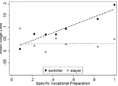
Figure 1:The relationship between the wage-loss after displacement and specific vocational preparation (SVP) is shown. I differentiate between workers who report to have switched occupations after displacement (black circles) and workers who stayed in the same occupation (gray triangles). The lines visualize weighted linear fits. It is apparent that the cost of switching occupations – what I refer to asmobility cost
– is strongly increasing in SVP. The fact that a similar relation is not observable for occupation stayers is reassuring evidence that the driving force is indeed the loss of occupation-specific human capital of switchers. Data on SVP comes from the the revised fourth edition of the Dictionary of Occupational Titles (1991). Data on wage-losses comes from the Current Population Survey Displaced Workers Supplement (CPS-DWS).
occupation a worker is trained in, the higher is therefore the mobility cost this worker is facing when switching
occupations. One contribution of this paper is to document that this relation is strongly confirmed in the data,
see Figure 1.
Secondly, I exploit geographic variation by using local labor market information from the U.S. Census. Local
labor markets differ regarding theirthickness. In a thick labor market it will be relatively easier to find a job
that matches a worker’s skill-set, even when highly specialized; mobility cost are therefore less likely to be
binding. I use two alternative measures to operationalize market thickness. My first measure is the size of
the local labor force. If workers and firms are heterogeneous in their skill endowments and requirements, an
increase in trading partners increases the probability that a worker can find a vacancy that matches his skills.
My second measure is the industrial diversity of the local labor market. In a diverse market, employment (and
different industries, in a diverse market it is more likely that at any given time there is a vacancy matching a
given worker skill.
Based on these two sources of variation, I construct the following test. I use data from the Current Population
Survey Displaced Worker Supplement (CPS-DWS) that contains information on completed unemployment
spells of workers displaced between 1983 and 2012 in the U.S. labor market. I examine the sample of displaced
workers who managed to find a job in the same occupation they worked in before. I then compare the
unemployment spells of more and less specialized workers in thin and thick local labor markets. If wait
unemployment matters, workers with more specific training should have relatively longer spells in thin markets
where mobility costs are likely to be binding. In thick markets, on the other hand, the difference should be
smaller or even non-existent.
My empirical results are in line with this hypothesis. For example, based on my regression results, I find
that in the thick New York metropolitan area labor market a industrial engineer who finds reemployment as
a industrial engineer goes through an unemployment spell that is about 3 weeks longer than a waiter who
finds reemployment as a waiter. On the other hand, in the relatively thinBakersfield, CAmetropolitan area a
industrial engineer sits through an unemployment spell that is almost 9 weeks longer than that of a waiter to
find a job in his old occupation. The differential unemployment spell is therefore about 6 weeks.
My interpretation of this finding is that inBakersfield, CAit is relatively more difficult to find reemployment
in the same occupation and therefore to transfer human capital to the next job. Since waiters only made
small investments in occupation-specific training they prefer switching occupations to going through a long
unemployment spell. Industrial engineers, on the other hand, have substantial occupation-specific training and
would suffer high wage-losses when switching occupations. They are therefore willing to go trough relatively
longer unemployment spells in order to find reemployment as industrial engineers.
I find that the occupation switching behavior of workers is consistent with this interpretation. While 60% of
industrial engineers find reemployment as industrial engineers, only 30% of waiters stay in their occupation in
the New York metropolitan area and only 19% in the thinBakersfield, CAlabor market. Moreover, based on a
difference-in-difference-in-differences approach, I document that long unemployment spells can only be found
for occupation stayers but not for occupation switchers. Since my estimation strategy allows me to control
for occupation- (and local-labor market) fixed effects, I can exclude that my results are driven by any inherent
differences between occupations.
Finally, I push the exercise further and use a worker’s specific vocational preparation as an instrument in a
(two-sample) two-stage least squares (TS2SLS) regression to obtain direct estimates of how mobility cost affect
increases in unemployment duration.
My results have important macroeconomic implications. Using a back-of-the-envelope calculation I find
that there would be between 9% and 18% less unemployment in the United States if human capital would be
transferable and switching occupations would not entail any mobility cost. Moreover, I argue that my findings
might offer important insights for the design of an optimal unemployment insurance system.
1.1. Related Literature
The idea that specificity of human capital can lead to long spells of wait unemployment is not new. To the
best of my knowledge, Murphy and Topel (1987) are the first to mention this channel explicitly. In particular,
they note that it is compatible with the observation that increased unemployed tends to go along with reduced
inter-sectoral mobility. This finding is strong evidence against sectoral-shift theories of unemployment as, for
example, proposed by Lilien (1982).
One strand of literature formalizes this idea in models where workers can undergo spells of “rest
unemploy-ment.” Jovanovic (1987), Hamilton (1988), King (1990), Gouge and King (1997), and more recently Alvarez and
Shimer (2008) extend the basic island model by Lucas Jr. and Prescott (1974). When a worker is subject to an
adverse shocks that lowers his wage he might rationally prefer not to work and to wait for better times instead
of undertaking a costly search for a better industry or occupation on another “island.” A sharp difference to
my framework is that in models of rest unemployment wages always fully adjust and clear markets. Rest
unemployment exists because workers have a utility from resting that might dominate working at the current
market wage. In my framework, on the other hand, the extent of wage adjustments is a critical factor in driving
unemployment. Workers are never voluntarily unemployed but they are queuing in order to put their human
capital to optimal use.
There is an older literature on transitional or wait unemployment that most resembles the concept of
un-employment I have in mind. The basic idea is that due to rigidities there are good and bad jobs that pay
workers of equal ability different wages. A fraction of workers rationally decide to queue and go through long
unemployment spells in order to get one of the highly paid jobs. This creates unemployment. Recently Alvarez
and Shimer (2008), based on ideas by Summers et al. (1986), claim that wage dispersion caused by unions leads
to substantial unemployment. In a classical paper Harris and Todaro (1970) identify wage differentials between
rural and urban jobs as a source of wait unemployment. Wait unemployment in my framework is different
inasmuch that workers are not queuing in order to seize rents but because they want to preserve valuable
specific human capital.
by analyzing earnings losses of displaced workers. Early papers in this literature tried to estimate the cost
of losing firm-specific capital (Abraham and Farber, 1987; Altonji and Shakotko, 1987; Kletzer, 1998; Topel,
1991). Neal (1995) and Parent (2000) analyzed the costs of changing industry after displacement. More recently,
there is growing evidence that human capital is mostly occupation- and not industry-specific (Kambourov and
Manovskii, 2009). I contribute to this literature by showing that the cost of switching differs substantiallyacross
occupations; leaving an occupation is more costly for workers who underwent lengthy and highly specific
occupational training (e.g., physicians) than for workers in occupations that makes use of mostly general skills
(e.g., waiters).
This paper also builds on a literature that explores the link between local labor market thickness, the quality
of job matches, and worker mobility. Helsley and Strange (1990) were the first to formalize the idea that, if
workers and firms (vacancies) are heterogeneous in their skill endowments and requirements, an increase in
trading partners increases the probability that a worker can find a vacancy that matches his skills. Thicker labor
markets therefore imply better job match quality and higher labor productivity. A consequence of this result is
that local labor market thickness also affects worker mobility. For example, both Wheeler (2008) and Bleakley
and Lin (2012) find evidence that workers early in their careers residing in thick labor markets are more likely
to change industries and occupations, presumably because they experiment with different types of work to
find out what job matches their skills best. More experienced workers, on the other hand, try to evade the
loss of specific human capital. Since the likelihood that a similar job is available in a thick market is relatively
high, these workers are thereforelesslikely to switch occupation and industry in thick local labor markets. My
findings are consistent with this evidence. The present paper adds to this literature by using the insight that the
likelihood to find re-employment in a similar job is increasing in local labor market thickness in the estimation
strategy
Finally, this paper contributes to the literature on labor market mismatch and structural unemployment.
This research has attracted increasing interest in recent times due to high and persistent unemployment rates
during and after the Great Recession of 2008 and because of claims that “structural factors” are behind this
development (Kocherlakota, 2010). Sahin et al. (2014) combine unemployment records with data on posted
vacancies to calculate mismatch unemployment in the U.S. labor market. They find that mismatch across
industries and occupations explains at most one-third of the increase of unemployment in the Great Recession
while geographic mismatch does not play a role. Barnichon and Figura (2011) use CPS data to explore the
effect of mismatch on matching efficiency. They find that lower matching efficiency due to mismatch can have
significant detrimental effect for unemployment in recessions. Herz and van Rens (2015) push the analysis a step
importance. This paper is complementary to this literature since I quantify evidence of how on very specific
channel – workers “waiting” for reemployment since they made specific investments ex-ante – contributes to
mismatch unemployment.
The remainder of this article proceeds as follows. In Section 2, I describe the different data sources that I use for
estimation. I discuss the basic estimation framework in Section 3. In Section 4, I estimate the relation between
SVP and mobility cost. Estimates of wait unemployment are presented in Section 5. I discuss the macroeconomic
implications of wait unemployment in Section 6. Firstly, using a “back-of-the-envelope” calculation I show
the importance of wait unemployment for aggregate unemployment in the United States. Secondly, I discuss
potential implications for the design of an optimal unemployment insurance system. Section 7 concludes. A
stylized model that formally shows the relation between market thickness and wait unemployment is presented
in the appendix.
2. Data and Measurement
2.1. Displaced Workers
My primary data set is the Current Population Displaced Workers Supplement (CPS-DWS) that has been widely
used for research on earnings-losses of displaced workers.1 The CPS-DWS was part of the CPS in January 1988,
February 1994, 1996, 1998, and 2000, and in January 2002, 2004, 2006, 2008, 2010, and 2012. CPS respondents are
asked whether they lost a job in the three years prior to the survey date (five years in 1988). Those individuals
who report having lost a job are part of the CPS-DWS and asked follow-up questions. This ex-post design is the
comparative advantage of the CPS-DWS because it allows the researcher to observecompletedunemployment
spells and provides information about a worker’s old and new job. In particular, job-losers are asked about both
their pre- and post-displacement weekly earnings, their pre- and post-displacement occupation,2 reasons for
displacement, and about the length of their initial unemployment spell.3 I refer the reader to the data appendix
A.2 for more information about the CPS-DWS and the exact sample that I use in this study.
1Some of the classic papers are Topel (1990), Gibbons and Katz (1991), Carrington (1993), Neal (1995), Farber et al. (1993), and Farber
et al. (1997).
2Occupation codes used in the CPS underwent several changes between 1988 and 2012. I therefore construct 384 time-consistent
occupation codes by using the conversion tables provided by Meyer and Osborne (2005).
3The exact wording of the question is “After that job ended, how many weeks went by before you started working again at another
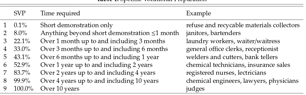
Table 1:Specific Vocational Preparation
SVP Time required Example
1 0.1% Short demonstration only refuse and recycable materials collectors
2 8.0% Anything beyond short demonstration≤1 month janitors, bartenders
3 22.1% Over 1 month up to and including 3 months laundry workers, waiter/waitress
4 33.0% Over 3 months up to and including 6 months general office clerks, receptionist
5 43.1% Over 6 months up to and including 1 year welders and cutters, bank tellers
6 52.9% Over 1 year up to and including 2 years chemical technicians, insurance sales
7 83.7% Over 2 years up to and including 4 years registered nurses, lectricians
8 99.9% Over 4 years up to and including 10 years chemical engineers, lawyers, physicians
9 100.0% Over 10 years judges
Notes: Definitions of the various levels of specific vocational preparation from the 1991 revised fourth edition of the Dictionary of Occupational Titles are reported. The first column shows the original (ordinal) variable. The second column shows the transformed (cardinal) variable. The latter was generated by constructing an empirical cumulative distribution function of SVP based on the 1995 basic monthly CPS data. For example, 52.9% of the workforce in 1995 were employed in occupations requiring at most 2 years of specific vocational preparation. Note that there is only one occupation in the highest category (judges) and one in the lowest category (refuse and recycable materials collectors).
2.2. Specific Vocational Preparation
My identification strategy requires a measure of the occupation-specific human capital a worker invested in.
I operationalize this by drawing on the “specific vocational preparation” (SVP) required to work in a given
occupation provided by the revised fourth edition of the Dictionary of Occupational Titles (DOT) published by
the U.S. Department of Labor in 1991. SVP is defined as “the amount of lapsed time required by a typical worker
to learn the techniques, acquire the information, and develop the facility needed for average performance in
a specific job-worker situation.”4 The variable that I use in this paper can be interpreted as the share of the
employed workforce that works in occupations with equal or smaller required specific vocational preparation.
See Table 1 for a description of the variable. I refer the reader to the data appendix for more information on the
construction of the variable.
2.3. Market Thickness
My identification strategy exploits that mobility cost should only matter when workers are forced to switch
occupations and mobility is necessary. To capture this source of variation empirically, I exploit that in athick
labor market it is more likely for a worker to find a vacancy that matches his skill endowment (see, e.g., Helsley
and Strange (1990) and Section 4.2.1 of Moretti (2011) for a survey). Switching occupations is therefore less
likely to be necessary.
I follow a popular approach in labor economics by assuming that local labor markets are well captured by
the concept of Metropolitan Statistical Areas (MSA) as defined by the Office of Management and Budget (OMB)
(e.g. Card, 2001; Mazzolari and Ragusa, 2011).5
I operationalize the concept of market thickness in two alternative ways. In both cases, the data comes from
the Integrated Public Use Microdata Series (IPUMS-USA) 5% sample of the U.S. Census for the years 1990 and
2000 (Ruggles et al., 2010).6
2.3.1. Market Size
The main measure of market thickness that I use in this paper is the size of an MSA’s labor force, SIZEm.
The motivation is that if workers and firms (vacancies) are heterogeneous in their skill endowments and
requirements, an increase in trading partners increases the probability that a worker can find a vacancy that
matches his skills. I refer the reader to the model in appendix A.1 for a more formal explanation of this
mechanism.
2.3.2. Industrial Diversity
As an alternative measure, I use the (inverse) industry fractionalization of a local marketmthat is equivalent to
the Herfindahl concentration index.7 The measure is formally defined as
1−DIVERSITYm =X
k
τ2mk (1)
whereτmkis the employment share of industrykin local labor marketm. It captures the probability that two
individuals who are randomly sampled from local labor marketmare employed in the same industry.
The motivation for using this measure is based on two observations. Firstly, as I report in detail in appendix
A.3, most occupations can be found in many different industries. Secondly, as I document in Section 4, as long
as workers stay in the same occupation, workers can switch industries without suffering a wage-loss.8 That is,
SVP captures purely occupation-specific training that is transferable across industries.
5Competing concepts are to use U.S. states (Topel, 1986; Herz and van Rens, 2015), counties (Gould et al., 2002), or so-called commuting
zones (Tolbert and Killian, 1987; Tolbert and Sizer, 1996; Autor et al., 2013). See the appendix A.2.1 of Dorn (2009) for a detailed discussion of local labor market concepts.
6There are some challenges to matching the CPS-DWS data to U.S. Census data. Between 1988 to 2012, the CPS-DWS uses three
different MSA classifications. In 1988 and 1992 it uses the U.S. Office of Management and Budget (OMB) 84 definitions, from 1994 to 2004 the OMB 93 definitions, and from 2006 on the OMB 2003 definitions. Throughout this paper I use the OMB 2003 classification by using a “geographic relationship file” provided by the Census that can be found athttps://www.census.gov/population/ metro/data/other.html.
7Measures of fractionalization have been widely used in economic research, in particular to analyze the impact of ethnic diversity on
corruption, conflict, and various economic or political outcome variables (e.g., Mauro, 1995; Easterly and Levine, 1997; Alesina et al., 1999; Miguel and Gugerty, 2005).
8For example when an electrician is switches occupations and works as a waiter, he will lose his specific training. However, when a
In a market with highDIVERSITYm, employment – and therefore vacancies – is evenly spread across many
industries. Assuming that industries’ vacancy posting is subject to random fluctuations that are not perfectly
correlated, this implies that the likelihood that at a given time there is no opening for a specific occupation in
the local market is decreasing inDIVERSITYm.9 The probability that a worker can find a vacancy that matches
his skills is therefore increasing inDIVERSITYm. I again refer the reader to appendix A.1 for a more formal
explanation of the mechanism.
To facilitate the interpretation of the estimates, I transform both variables by generating empirical cumulative
distribution functions. The new variables can then be interpreted as, firstly, the percentage of the total U.S.
metropolitan labor force that resides in a MSA of equal or smaller size, and secondly, the percentage of the U.S.
metropolitan workforce that lives in a MSA with equal or lower industrial diversity. For convenience, in the
following I refer to bothSIZEmandDIVERSITYmas measures of labor marketthickness.
3. Basic Estimation Framework
The relation between wait unemployment, mobility cost, and specific vocational preparation can be described
by the following two regression equations. The first regression is estimated on the sub-sample of “switchers,”
that is, workers whose pre- and post-displacement occupation isnotthe same:
MCijt=α1+α2SVPj+θ′Xi+ǫijt (2)
The second regression is estimated on the sub-sample of “stayers,” that is, workers whose pre- and
post-displacement occupation is the same:
UNEMijt=β1+β2MCijt+θ′Xi+ηijt (3)
MCijt is the mobility cost of a displaced worker i measured as the (expected) wage-loss (the log-earnings
difference) he would suffer when leaving his pre-displacement occupationj.
The first regression captures the effect of specific human capital on mobility cost, visualized in Figure
1: conditional on switching to another occupation after displacement, there is a strong positive correlation
between the extent of occupation-specific training a worker invested in and the wage-loss he experiences. This
impliesα2>0. As described in Section 2.2, I proxy the occupation-specific training by the length of the required
specific training of the worker’s last occupation,SVPj.
The second regression formalizes the idea of wait unemployment. The higher the (expected) mobility cost
MCijta worker is facing, the longer the unemployment spellUNEMijthe is willing to go through in order to evade
switching occupations. UNEMijtis measured as the natural logarithm of 1 plus the weeks of unemployment:
log(1+weeksijt).10 If wait unemployment matters, it should holdβ2 >0.
All regressions also include a vector of worker-specific demographic control variables Xi to reconcile the
model with the data and account for the fact that in reality workers differ among many more dimensions than
the ones captured by the simple model. Regressions include year-of-displacement dummies, four education
dummies (dropout, high-school, some college, college or more), a female dummy, a non-black dummy, and
potential experience (quadratic). Importantly, all regressions also include the tenure on the pre-displacement
job (cubic). The wage-loss captured by coefficientα2in regression (2), for example, is therefore purely due to
specific vocational training, not due to job tenure. As explained in the data appendix A.2, it is also important to
take into account whether a worker was displaced due to plant closing. In order to capture this, all regressions
include a plant closing dummy that is also interacted with worker-specific demographic variables.
I report estimates of equation (2) in the next section. I then turn to equation (3) in Section 5 .
4. Specific Human Capital and Mobility Cost
Regression equation (2) relates to a big literature in labor economics that studies the specificity of human capital
by analyzing earnings losses of displaced workers. Early papers in this literature try to shed light on the degree
of firm-specificity of human capital (Abraham and Farber, 1987; Altonji and Shakotko, 1987; Kletzer, 1998;
Topel, 1991) while Neal (1995) and Parent (2000) analyze the costs of switching industry. More recently, there is
growing evidence that human capital is actually mostly occupation-specific (e.g., Kambourov and Manovskii,
2009).
Here I contribute to this literature by showing that the extent of human capital lost upon leaving an occupation
also differs substantially across occupations. In particular, I show that the SVPj of an occupation is a good
predictor of the extent of human capital lost upon switching. For example, a physician who underwent lengthy
and highly specific occupational training will lose a substantial amount of human capital upon leaving his
occupation. This is reflected in a high wage-loss. On the other hand, for workers in occupations that make
use of mostly general skills (e.g., bartender, cashier) switching occupations entails only a limited loss of human
capital resulting in only marginal wage-losses.
Column (1) of Table 2 reports estimates of equation (2). The coefficient onSVPj is positive and significant
10The results in this paper are robust to instead usinglog(weeks
Table 2:Mobility Cost and SVP
(1) (2) (3) (4) (5) (6) (7)
SVPj 0.144*** 0.00613
(0.0266) (0.0240)
SWITCHERijt 0.0778*** -0.0241 0.00321 -0.0478 -0.0421
(0.0117) (0.0263) (0.0231) (0.0301) (0.0272) SVPj×SWITCHERijt 0.160*** 0.131*** 0.200*** 0.188***
(0.0330) (0.0295) (0.0416) (0.0363)
IND SWITCHERijt 0.00900
(0.0583)
SVPj×IND SWITCHERijt 0.0223
(0.0731)
Observations 7,918 12,355 12,355 12,355 4,832 8,604 4,046
R-squared 0.071 0.127 0.129 0.067 0.146 0.152 0.193
Occupation fixed effects no yes yes no yes yes yes
Sample
Occupation switchers only yes no no no no no no
Occupation stayers only no no no no no no yes
Plant closing only no no no no yes no no
No advance notice only no no no no no yes no
Notes: Column (1) reports estimates of regression (2) whereas columns (2)-(7) report estimates of variations of regression equation (4). The method of estimation is least squares. The dependent variable is the wage-loss defined as the log-difference between deflated weekly earnings on the
pre-displacement jobs and the current job. All regressions include year-of-pre-displacement dummies, four education dummies (dropout, high-school, some college, college or more), a female dummy, a non-black dummy, potential experience (quadratic), tenure on the pre-displacement job (cubic), and con-trols that capture whether displacement was due to plant closing. Only the sub-sample of displaced workers who report that the current job was the
first job after displacement is used for estimation. As noted at the bottom of the table, the sample is further restricted in columns (1) and columns (5)-(7). Standard errors clustered at the occupation level are reported in parenthesis. ***, **, and * indicate significance at the 1%, 5%, and 10% levels.
at the 1% level. As described in Section 2.2, SVPj is the share of the workforce that works in occupations
requiring less or equal specific vocational preparation than occupation j. The estimates therefore imply that
every 10 percentage point increase in the SVP distribution leads to a 1.4 percentage point increase in the expected
wage-loss when switching occupations after displacement. This magnitude is economically important.
A problem with this simple specification is that I cannot for occupation fixed effects. It is therefore possible that
the estimated positive coefficient onSVPjresults from unobserved occupation characteristics that systematically
vary withSVPj. My baseline is therefore the modified regression
MCijt=α1 SWITCHERijt+α2 SWITCHERijt×SVPj+χj+θ′Xi+ǫijt. (4)
This regression includes occupation fixed effectsχjand is estimated on the whole sample of displaced workers,
including both occupation stayers and switchers. SWITCHERijt is a dummy variable that indicates whether
individualiwith pre-displacement occupation jfound a job in the same occupation.
relative to stayers across occupations characterised by low and high specific vocational preparation. The
estimate of interest is therefore the coefficient on the interactionSWITCHERijt×SVPj. Note that the mean effect
ofSVPjis captured by the occupation fixed effectsχj.
Regression estimates are shown in columns (2) to (7) of Table 2. In column (2) I report estimates from a
simplified model that does not includeSWITCHERijt×SVPjas a regressor. Switching occupations goes along
with a wage-loss as the coefficient onSWITCHERijtis highly significant. This finding is not new (Kambourov
and Manovskii, 2009, e.g.).
I contribute to this literature by showing that this simple model masks substantial heterogeneities. In the
full model in column (3) the coefficient on the interactionSWITCHERijt×SVPj is estimated to be positive and
highly significant while the coefficient on the main effectSWITCHERijt is not significantly different from zero
anymore. This implies that switching occupationsper se does not lead to a wage-loss. However, switching
iscostly for workers who made substantial investments in specific vocational preparation. The magnitude is
economically important: the expected differential wage-loss is increasing by about 1.6 percentage points for a
10 percentage points increase ofSVPj. This implies, for example, that the differential expected wage-loss upon
leaving an occupation is about 10 percentage points higher for an electrician (83% percentile) compared to a
waiter (22% percentile).
Column (4) reports estimates when occupation fixed effects are not included and the mean effect of SVPj
is therefore identified. Interestingly, the estimated coefficient onSVPj is not significantly different from zero,
meaning that conditional on staying in the same occupation, the wage-loss workers suffer doesnotdiffer by
the required specific vocational preparation of an occupation. This is reassuring evidence thatSVPjis indeed
mostly capturing occupation-specific training and not firm- or match-specific human capital.
Columns (5) and (6) show results when the sample is restricted further. Column (5) reports estimates when
only workers who report having been displaced due to plant closing are included. As discussed in the data
appendix A.2, this sample is arguably preferable to my overall sample because in this case weak performance
on the job cannot have been the reason for displacement and therefore estimates will be less subject to criticism
regarding selection bias. The coefficient on the interaction gets larger, implying that estimates based on my
baseline sample might be subject to some selection effects.
In column (6) the sample is restricted to workers who did not receive an advance notice of displacement, see
appendix A.2. Again, results are larger than in the baseline. This suggests that the benefits of on-the-job-search
are the higher the more specific a worker’s training is. In order to account for this effect, I will use the sub-sample
of workers who were not noticed in advance of their displacement as my baseline sample when estimating
In column (7) I restrict the sample to workers who did not switch occupations. At the same time I add a
dummy that captures whether a worker stayed in the sameindustryafter displacement or not. The coefficient
on the interaction and the mean effect are both not significantly different from zero. This corroborates evidence
from column (4):SVPjindeed captures human capital that is occupation- but notindustry-specific.
5. Estimates of Wait Unemployment
5.1. Reduced Form Estimates
Equation (3) captures the concept of wait unemployment: there is a trade-offbetween unemployment duration
and mobility cost. Switching occupations and leaving behind occupation-specific human capital can entail high
wage-losses. Facing such mobility costs workers might be willing to accept long unemployment spells in order
to evade switching and secure reemployment in their old occupation instead. My objective is to empirically
quantify this trade-off.
A problem hindering estimation is that the (expected) wage-loss a worker faces upon leaving his
pre-displacement occupationMCijtis by definition not observed for the sub-sample of occupationstayersequation (3)
is estimated on. Furthermore, any reasonable measure of mobility costMCijtand the worker’s unemployment
durationUNEMijtare likely to be simultaneously determined. That is, not only might mobility cost incentivize
workers to sit through long spells of wait unemployment, but long unemployment spells might also weaken
the bargaining position of workers and therefore lead to lower wages and lower mobility cost. This would
lead to a downward bias in the estimation results. I therefore combine equations (2) and (3) into the following
reduced form equation:
UNEMijt=γ1+γ2 SVPj+θ′Xi+νijt (5)
Unlike the mobility costMCijt,SVPjis directly observable from theDictionary of Occupational Titlesas explained
in detail in Section 2. Moreover,SVPjis arguably a pre-determined variable and endogeneity should therefore
be much less of a problem.
However, a second challenge for estimation remains. As before the (likely) presence of occupation fixed
effects might result in biased estimates. Occupations associated with high mobility cost might differ in other
– potentially unobserved – characteristics from occupations subject to low mobility cost. For example, service
occupations might require only few specific vocational preparation and workers therefore are likely to face
small mobility cost upon switching occupations. Nevertheless, these workers might have above-average
cross-occupation variation for identification it is difficult to distinguish the effect of variation in mobility cost (I
am interested in) from variation in other unobserved occupation characteristics that systematically vary with
mobility cost.
To avoid potential omitted variable bias I therefore rely onwithin-occupation differences for identification.
To do so I exploit geographic variation: as formalized in the appendix, the higher thethicknessa local labor
market, the less likely is it that displaced workers need to switch occupations; potential mobility cost are less
likely to be binding. I estimate the following regression equation on the sub-sample of occupation stayers:
UNEMijmt=γ1THIN MARKETm+γ2THIN MARKETm×SVPj+χj+θ′Xi+νijmt (6)
The mean effect ofSVPjis captured by the occupation fixed effectsχj. The estimation strategy follows the same
logic as a standard difference-in-differences approach. However, note that bothTHIN MARKETmandSVPjare
continuous measures. The hypothesis is that highly specialized workers sit through long unemployment spells
in order to evade switching occupations. Since in a thin marketmit is less likely to be able to find a job in the
same occupation, this effect should be increasing inTHIN MARKETm. The estimate of interest is therefore the
coefficient on the interactionTHIN MARKETm×SVPj. Under the hypothesis that wait unemployment is an
important driving force of unemployment it should holdγ2 >0.
5.1.1. Main Results
Table 3 shows results when market thickness is operationalized as the size of the local labor force. Again, all
specifications contain typical demographic controls and tenure on the previous job. Furthermore, occupation
fixed effects, year-of-displacement fixed effects, state fixed effects, and controls capturing whether displacement
was due to plant closing are part of all specifications. Mean effects and the constant are estimated but not shown.
Results in column (1) indicate a coefficient estimate for the interaction term that is positive and statistically
significant at the 1-percent level. Adding a linear state time trend in column (2) does not change the results.
Adding MSA fixed effects in (3) slightly decreases the size of the coefficient.11 The estimates imply that there is a
significant differential effect of the required specific vocational preparation of an occupation on unemployment
duration. The thinner a local market is, the stronger is the effect ofSVPj on the length of the unemployment
spell.
The difference-in-differences setting makes it difficult to interpret the magnitude of the estimated effect. I
therefore follow Rajan and Zingales (1998) and report adifferential unemployment spellfor each specification in
11State fixed effects do not completely drop out in this specification because some metropolitan areas span more than one state. Results
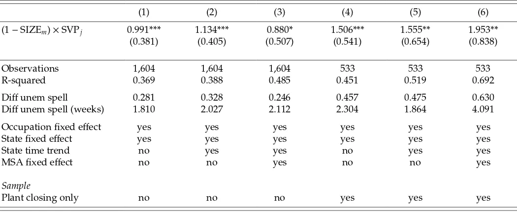
Table 3:Reduced Form Estimates: Market Size
(1) (2) (3) (4) (5) (6)
(1−SIZEm)×SVPj 0.991*** 1.134*** 0.880* 1.506*** 1.555** 1.953**
(0.381) (0.405) (0.507) (0.541) (0.654) (0.838)
Observations 1,604 1,604 1,604 533 533 533
R-squared 0.369 0.388 0.485 0.451 0.519 0.692
Diffunem spell 0.281 0.328 0.246 0.457 0.475 0.630
Diffunem spell (weeks) 1.810 2.027 2.112 2.304 1.864 4.091
Occupation fixed effect yes yes yes yes yes yes
State fixed effect yes yes yes yes yes yes
State time trend no yes yes no yes yes
MSA fixed effect no no yes no no yes
Sample
Plant closing only no no no yes yes yes
Notes:The regressions are least squares estimates of equation (6). The dependent variable is the length of the unemployment spellUNEMijmt, measured
as the natural logarithm of 1 plus the weeks of unemployment:log(1+weeksijt). I operationalize market thickness using the size of the local labor force.
Thedifferential unemployment spellreports the relative increase in the unemployment duration of a displaced worker with high SVP relative to a worker with low SVP (75th vs. 25th percentile) when located in a thick vs. thin local labor market (75th vs. 25th percentile). All regressions include
year-of-displacement dummies, four education dummies (dropout, high-school, some college, college or more), a female dummy, a non-black dummy, potential experience (quadratic), tenure on the pre-displacement job (cubic), and controls that capture whether displacement was due to plant closing. Only the sub-sample of displaced workers who report not to have changed occupations after displacement, whose current job was the first job after displacement,
who were not noticed in advance of their displacement, and who did not move after displacement is used for estimation. In columns (4) to (6) the sample is further restricted to workers who report to have been displaced due to plant closing. Standard errors clustered at the occupation level are reported in parenthesis. ***, **, and * indicate significance at the 1%, 5%, and 10% levels.
Table 3. Consider two unemployed workers who have been displaced from occupations at the 25th and 75th
SVP percentile, respectively. Think of the first as a waiter and of the latter as an electrician. According to the
U.S. Census, only 25% of the labor force reside in metropolitan areas bigger than the Washington metropolitan
area, the 6th biggest MSA in the United States. On the other hand, 75% reside in MSAs bigger thanBakersfield,
CA. For example, the estimates reported in columns (1) of Table 4 imply that the unemployment spell of the
electrician would increase by 28.1 percentage points more than that of the waiter if both were re-located from
the thick labor market in the Washington metropolitan area toBakersfield, CA.12In levels, this corresponds to
about two weeks.13
In columns (4) to (6) I restrict the sample to workers who report having been displaced due to plant closing
only. As discussed in the data appendix A.2, this sample is arguably preferable to my baseline sample that
also includes workers who lost their job due an abolished shift and “insufficient work.” If displaced workers
have systematically lower ability and workers with lower ability in turn have lower specific vocational training,
12This number can be calculated from the estimated coefficients given in column (1) of Table 3 asexp((0.75−0.25)2×0.991)−1≈28.1%. 13I follow Duan (1983) to retransform the dependent variable in logs back to levels. See also Section 3.6.3 in Cameron and Trivedi
Table 4:Reduced Form Estimates: Industrial Diversity
(1) (2) (3) (4) (5) (6)
(1−DIVERSITYm)×SVPj 1.051*** 1.210*** 1.155** 1.584*** 1.811*** 1.475**
(0.385) (0.432) (0.519) (0.467) (0.536) (0.685)
Observations 1,604 1,604 1,604 1,024 1,024 1,024
R-squared 0.369 0.388 0.487 0.356 0.392 0.508
Diffunem spell 0.301 0.353 0.335 0.486 0.572 0.446
Diffunem spell (weeks) 2.077 2.301 2.879 3.202 3.346 4.354
Occupation fixed effect yes yes yes yes yes yes
State fixed effect yes yes yes yes yes yes
State time trend no yes yes no yes yes
MSA fixed effect no no yes no no yes
Sample
Occs. in many inds. only no no no yes yes yes
Notes:The regressions are least squares estimates of equation (6). The dependent variable is the length of the unemployment spellUNEMijmt, measured
as the natural logarithm of 1 plus the weeks of unemployment:log(1+weeksijt). I operationalize market thickness using the my measure of industrial
diversity. In columns (6) to (10), I exclude occupations that are concentrated in few industries. Thedifferential unemployment spellreports the relative increase in the unemployment duration of a displaced worker with high SVP relative to a worker with low SVP (75th vs. 25th percentile) when located
in thick vs. thin local labor market (75th vs. 25th percentile). All regressions include year-of-displacement dummies, four education dummies (dropout, high-school, some college, college or more), a female dummy, a non-black dummy, potential experience (quadratic), tenure on the pre-displacement job (cubic), and controls that capture whether displacement was due to plant closing. Only the sub-sample of displaced workers who report not to have
changed occupations after displacement, whose current job was the first job after displacement, who were not noticed in advance of their displacement, and who did not move after displacement is used for estimation. In columns (4) to (6) occupations present in only few industries are excluded. Standard errors clustered at the occupation level are reported in parenthesis. ***, **, and * indicate significance at the 1%, 5%, and 10% levels.
then this might result in an underestimation of the effect ofSVPjon wait unemployment. Moreover, using this
sample I can exclude that estimates are biased because workers expect to be recalled to their old job. Indeed,
the estimated coefficients are larger than in the baseline sample and, in spite of the smaller sample, remain
significantly different from zero. This suggests that estimates using the baseline sample represent a lower
bound on wait unemployment.
Industrial Diversity
Table 4 reports results when market thickness is operationalized as the industrial diversity of the local labor
market instead of the size of its labor force, see Section 2.3. Columns (1) to (3) document that the coefficient of
interest remains significantly different from zero and of similar size to the estimates reported in Table 3.
A potential concern regarding the use of the industrial diversity measure is that the employment of some
occupations is heavily concentrated in only few industries. For example, according to the 1990 U.S. Census,
83% of bakers are employed in the three industriesGrocery stores,Bakery products, andRetail bakeries. For some
Table 5:Reduced Form Estimates: Occupation Switching
(1) (2) (3) (4) (5) (6) (7) (8) (9) (10)
SVPj -0.125* -0.127* -0.0176 -0.0209 0.0980 0.100
(0.0700) (0.0699) (0.0826) (0.0835) (0.0684) (0.0678) (1-SIZEm)×SVPj -0.203** -0.199** -0.195** -0.159*
(0.0904) (0.0880) (0.0794) (0.0889)
(1-DIVERSITYm)×SVPj -0.442*** -0.450*** -0.447*** -0.412***
(0.104) (0.104) (0.105) (0.105)
Observations 4,372 4,372 4,372 4,372 4,372 4,372 4,372 4,372 4,372 4,372
R-squared 0.060 0.069 0.062 0.071 0.267 0.319 0.066 0.075 0.271 0.322
Occupation fixed effect no no no no yes yes no no yes yes
State fixed effect yes yes yes yes yes yes yes yes yes yes
State time trend no yes no yes yes yes no yes yes yes
MSA fixed effect no no no no no yes no no no yes
Notes:The regressions are least squares estimates of equation (7). The dependent variable is 0 if the pre- and post-displacement occupation of a dis-placed worker is the same and 1 if it is different. I operationalize market thickness using the size of the local labor force in columns (3) to (6) and as industrial diversity in columns (7) to (10). All regressions include year-of-displacement dummies, four education dummies (dropout, high-school, some college, college or more), a female dummy, a non-black dummy, potential experience (quadratic), tenure on the pre-displacement job (cubic), and controls that capture whether displacement was due to plant closing. The regression also controls for the length of the completed unemployment spell. The sample contains both workers who have and who have not changed occupations after displacement. The sample is restricted to workers whose current job was the first job after displacement, who were not noticed in advance of their displacement, and who did not move after displacement. Standard errors clustered at the occupation level are reported in parenthesis. ***, **, and * indicate significance at the 1%, 5%, and 10% levels.
employed inHotels and motelsand school teachers work inElementary and secondary schools. Occupations like
these should therefore not benefit from industrially diverse local labor markets.
To address this issue, I firstly document in appendix A.3 that such occupations are an exception and that
em-ployment in most occupations indeed spans many industries: the median worker is employed in an occupation
that can be found in 48 different industries. Secondly, the fact that occupations differ in the degree to which they
span different industries allows me to test an additional hypothesis: industrial diversity of a local labor market
should be especially important for occupations that span a higher number of industries and should therefore
have a relatively stronger effect on wait unemployment.
I explore this in columns (4)-(6) of Table 4 by excluding occupations that can be found in less than 24 different
industries (that is, I exclude occupations ranked within the lower two quintiles according to their industry-span).
In line with the hypothesis, the coefficient of interest increases substantially in size.
5.1.2. Occupation Switching
My interpretation of the results reported in Tables 3 and 4 is that workers endowed with specific human
capital face high mobility costs when switching occupations and are therefore willing to go through long
unemployment spells in order to find a job in the same occupation. If this is true, we would expect workers
difficult to find a job in the same occupation. I estimate the following regression equation:
SWITCHERijmt=δ1SVPj+δ2 THIN MARKETm+δ3THIN MARKETm×SVPj+θ′Xi+ωijmt (7)
(Pre-displacement) occupation fixed effects, year-of-displacement fixed effects, state fixed effects, and controls
capturing whether displacement was due to plant closing are part of all specifications. Columns (1) and (2) of
Table 5 report estimates of a simplified model that assumesδ2=0 andδ3 =0. I find that workers endowed with
more specific human capital are indeed more likey to stay in their pre-displacement occupation. In columns
(3) and (4) I show results of the full model that allows the effect of SVP to differ depending on the thickness of
the local labor market. The estimates are consistent with wait unemployment. SVP does not have an effect on
switching behavior in very thick labor markets ((1−SIZEm)=0) since being able to stay in the same occupation
is less difficult. The thinner the market, however, the more likely are workers with non-specific human capital
to switch. The effects are quantitatively important. To use the example from above, estimates in column (3)
imply that in the thick Washington metropolian area market a worker at the 25 percentile of SVP (a waiter) is
3.4% percentage points more likely to switch than one at the 75 percentile (an electrician). In the relatively thin
Bakersfield, CAmarket, however, this differene increases to 8.5 percentage points.14
In column (5) I include occupation fixed effects andSVPjis therefore no longer identified. The coefficient on
THIN MARKETm×SVPjremains almost unchanged and only becomes slightly smaller when MSA fixed effects
are added in column (6). The results become quantitatively stronger when the industrial diversity measure is
used in columns (7) to (10).
5.1.3. Triple Differences
One might argue that the estimates reported in Section 5.1.1 are compatible with other mechanisms than wait
unemployment. The interactionTHIN MARKETm×SVPjmight be just a proxy for another, unobserved channel.
In particular, workers with highly specific training might benefit disproportionally from thick labor markets
due to reasons not related to wait unemployment.
Here I therefore use the sample of both occupation stayers and switchers to construct another test. Wait
unemployment means that displaced workers sit through long unemployment spells in order to stay in the
occupation they have been trained for. If the long unemployment spells I observe in the data are indeed due
to wait unemployment, I should therefore observe these long spells only for occupation stayers, but not for
switchers. In this section I show that this is indeed the case with my data.
I estimate a difference-in-difference-in-differences regression on the sample including both occupation stayers
Table 6:Reduced Form Estimates: Triple Differences
(1) (2) (3) (4) (5) (6) (7) (8) (9) (10) (1-SIZEm)×SVPj 0.737** 0.750** 0.540 1.336** 1.424***
(0.356) (0.356) (0.357) (0.528) (0.546) SWITCHERijmt×(1-SIZEm)×SVPj -0.333 -0.408 -0.0922 -1.285 -1.115
(0.556) (0.551) (0.497) (1.006) (0.909)
(1-DIVERSITYm)×SVPj 0.716* 0.759** 0.636 1.294*** 1.163***
(0.365) (0.375) (0.386) (0.442) (0.445) SWITCHERijmt×(1-DIVERSITYm)×SVPj -0.982** -1.051** -0.939* -1.609** -1.634***
(0.487) (0.507) (0.517) (0.619) (0.560) Observations 4,372 4,372 4,372 1,365 1,365 4,372 4,372 4,372 3,048 3,048 R-squared 0.229 0.242 0.289 0.345 0.449 0.229 0.242 0.289 0.228 0.291 Total effect switchers 0.403 0.342 0.448 0.0509 0.309 -0.266 -0.292 -0.303 -0.315 -0.470 P-value 0.200 0.273 0.138 0.944 0.646 0.334 0.307 0.309 0.360 0.130 Occupation fixed effect yes yes yes yes yes yes yes yes yes yes State fixed effect yes yes yes yes yes yes yes yes yes yes State time trend no yes yes yes yes no yes yes yes yes MSA fixed effect no no yes no yes no no yes no yes
Sample
Plant closing only no no no yes yes no no no no no Occs. in many inds. only no no no no no no no no yes yes
Notes:The regressions are least squares estimates of equation (8). The dependent variable is the length of the unemployment spellUNEMijmt, measured as the
natural logarithm of 1 plus the weeks of unemployment:log(1+weeksijt). I operationalize market thickness using the size of the local labor force in columns (1)
to (5) and industrial diversity in columns (6) to (10). The row labeled “total interaction switchers” shows the sum of coefficients THIN MARKETm×SVPjand
SWITCHERijmt×THIN MARKETm×SVPj. All regressions include year-of-displacement dummies, four education dummies (dropout, high-school, some college,
college or more), a female dummy, a non-black dummy, potential experience (quadratic), tenure on the pre-displacement job (cubic), and controls that capture whether displacement was due to plant closing. The sample contains both workers who have and who have not changed occupations after displacement. The sample is restricted to workers whose current job was the first job after displacement, who were not noticed in advance of their displacement, and who did not move after displacement. In columns (4) and (5) the sample is further restricted to workers who report to have been displaced due to plant closing. In columns (9) and (10) occupations present in only few industries are excluded. Standard errors clustered at the occupation level are reported in parenthesis. ***, **, and * indicate significance at the 1%, 5%, and 10% levels.
and switchers by adding a third interaction to regression (6):
UNEMijmt=γ1 SWITCHERijmt+γ2THIN MARKETm×SVPj+γ3 THIN MARKETm×SWITCHERijmt
+γ4SWITCHERijmt×SVPj+γ5THIN MARKETm×SVPj×SWITCHERijmt+χj+θ′Xi+νijmt (8)
SWITCHERijmt is a dummy variable that indicates whether individual iwith pre-displacement occupation j
found a job in the same occupation. The coefficient on the interactionTHIN MARKETm×SVPjcaptures the effect
of mobility cost on unemployment duration whereas the coefficient onTHIN MARKETm×SVPj×SWITCHERijmt
is the differential effect on workers who report to have switched occupations.
Columns (1) to (5) of Table 6 report results when market thickness is operationalized as the size of the local
labor force. The coefficients for occupation stayers are slightly smaller in magnitude than in the baseline in
Table 3. As before, the results become stronger once the sample is restricted to workers who report having
been displaced due to plant closing only in columns (4) and (5). Importantly, the effect for switchers is never
significantly different from zero, see the row labeled “total effect switchers” in the table.15 As reported in
columns (6) to (10) of Table 6, the results also hold when market thickness is operationalized as industrial
diversity. As before, the results become stronger when occupations concentrated in few industries are excluded
from the sample in columns (9) and (10).
5.1.4. Geographic Mobility
Another potential concern is geographic mobility. Some workers might manage to stay in the same occupation
without going through a spell of wait unemployment by moving to another labor market. In Table 10 in the
appendix I report estimates of the regression equation
SWITCHERijmt=δ1MOVEDijmt+δ2MOVEDijmt×SVPj+χj+θ′Xi+ωijmt. (9)
MOVEDijmt equals 1 if a displaced worker reports to have moved cities after displacement and 0 otherwise.
I find that displaced workers who report to have moved cities are indeed more likely to stay in their
pre-displacement occupation, especially when endowed with high SVP. Geographic mobility reduces the number
of unemployed in slack local labor markets and therefore leads to a reduction of wait unemployment for the
remaining workers. Since, as explained in the data appendix, the estimates presented above are based on the
sample of displaced workers who report not to have moved cities after displacement they implicitly take the
effect of geographic mobility into account.16
5.2. Instrumental Variable Estimates
In the last section I showed evidence that workers endowed with more specific training are willing to go
through disproportionately long spell of unemployment in order to evade switching occupations. I now push
the analysis further and directly estimate the effect of mobility cost on wait unemployment captured by equation
(3). In order to do so, I make the additional identifying assumption thatSVPj affects unemployment duration
only through the mobility cost a worker is facing. I can then estimate equation (3) by usingSVPjas an instrument
for the mobility costMCijt.17 To control for occupation fixed effects, I use the same difference-in-differences
in their original occupation and only after learning that few vacancies are around decide to switch. One can also interpret this as a measurement problem. In the data workers only report in what occupation theyeventuallyfound a job and how many weeks it took them to find this job. It is not clear how the time spend searching was distributed among finding a job in their pre-displacement occupation vs. finding a job in another occupation.
16As suggested by an anonymous referee, there are some other tests one might construct in order to further explore whether observed
geographic mobility is in line with wait unemployment. For example, one would expect a higher probability of moving cities for high SVP workers displaced in thin labor markets. Unfortunately, the CPS Displaced Workers Supplement only contains the worker’s MSA of residence at the time of the interview, not at the time of displacement. The local labor market where a worker was displaced can therefore not be inferred for workers who report to have moved after displacement.
17Note thatSVP
approach as in regression (6). Based on equation (3), the second-stage can then be written as
UNEMijmt=β1THIN MARKETm+β2 THIN MARKETm×MCijmt+χj+θ′Xi+ηijmt. (10)
A challenge to use two-stage least squares in my setting is that mobility costMCijmtare only observed for the
sample of occupationswitcherswhile the dependent variable in equation (10) is the unemployment duration of
stayers. That is, the endogenous regressor and the dependent variable are not part of the same sub-sample.
As first shown in an influential article by Angrist and Krueger (1992), under certain conditions estimation
is still feasible by using the two-sample two-stage least squares (TS2SLS) procedure.18 The principal idea of
TS2SLS is that the first- and second-stage can be estimated on two separate samples as long as all control
variables and the instrument are present in both samples, and – as it is the case here – both samples have
been drawn from the same population. Since the distribution of observable characteristics might vary between
the samples of switchers and stayers, it is important to note that this is implicitly corrected for by the TS2SLS
estimator and estimates remain consistent (see footnote 1 in Inoue and Solon (2010)).
The estimate of interest in regression (10) is the coefficient on the interactionTHIN MARKETm×MCijmtwhere
the mobility costMCijmt is likely to be endogenous. I therefore useTHIN MARKETm×SVPjas an instrument
for this interaction.19 The first-stage regression on the sample of switchers is then given by
THIN MARKETm×MCijmt =α1THIN MARKETm+α2THIN MARKETm×SVPj+χj+θ′Xi+κijmt. (11)
The idea of this estimation approach is to use the wage-loss actually suffered by occupation switchers as a
predictor of the (unobserved) expected wage-loss stayers would have suffered in the case of switching. A
potential point of criticism is that switchers and stayers differ in unobservable characteristics and that the
realized wage-loss of a switcher might therefore be systematically different from the (unobserved) expected
wage-loss of an observationally equivalent stayer. However, note that – apart from the usual demographic
controls – both the first- and second-stage include occupation fixed effects. The assumption I make is therefore
weaker: I assume that thedifferentialwage-loss of switchers is a good predictor of the differential (expected)
wage-loss of stayers.
In order forTHIN MARKETm×SVPjto be a valid instrument it needs to be relevant, exogenous, and fulfill
the exclusion restriction. An instrument is relevant if it has sufficient explanatory power for the explanatory
variable, that is, ifcorr(THIN MARKETm×SVPj,THIN MARKETm×MCijmt) is not only marginally different
18See also Angrist and Krueger (1995), Inoue and Solon (2010), and Chapter 4.3 in Angrist and Pischke (2008).
19See Ozer-Balli and Sorensen (2010) for a discussion on how to use instrumental variables in linear regressions that include interaction
from zero. If this is not the case IV estimates are unlikely to be informative. This condition is testable and
– as shown below – indeed holds in my data. The instrument is also arguably exogenous becauseSVPj is a
pre-determined variable.
The exclusion restriction holds if, conditional on the control variables,THIN MARKETm×SVPj is
uncorre-lated with any other determinants of unemployment duration. The instrumentTHIN MARKETm×SVPjmust
affect the unemployment duration of a workers only through the interactionTHIN MARKETm×MCijmt. In
particular, one might argue that in a thick labor market there might be more opportunities for workers trained in
highly specific tasks, leading to relatively shorter unemployment spells. However, I argue that this is unlikely
given the evidence reported in Section 5.1.3: the fact that I find evidence of long spells for occupation stayers
but not for occupation switchers strongly suggests that the long spells indeed result from skilled workers trying
to evade switching occupations and not from simple differences in the matching technology.
5.2.1. Results
Table 7 presents two-sample two stage least squares estimates of the effect of mobility cost on unemployment
duration. The associated first-stage estimates on the sample of occupation switchers are shown in Table 11 in
the appendix. Columns (1) to (4) show results when market thickness is measured as the size of the local labor
force. As before, all specifications include the usual demographic controls, occupation fixed effects, state fixed
effects, and controls for plant closing. In column (2) I also allow for state-specific time trends. In the first two
specifications the coefficient on the interaction is positive and significant at the 5% level.20 As reported in Table
11 in the appendix, for both specifications the first-stage is relatively strong with an F-statistic on the instrument
of about 13, well above the threshold of 10 suggested by Staiger and Stock (1997). This indicates that weak
instruments should not be an important concern.
As for the reduced form estimates, I compute adifferential unemployment spellto make it easier to put
mag-nitudes into perspective. According to results in column (1), if a displaced worker facing a 10% mobility cost
would be located in the thinBakersfield, CAlabor market instead of the thick labor market of the Washington
metropolitan area, his unemployment spell would increase by 30%.21 In levels, this corresponds to about 2.5
weeks.
In column (3) I include MSA fixed effects. While the coefficient of interest is less precisely estimated and
not significantly different from zero, its magnitude is only slightly smaller compared to columns (1) and (2).
In column (4) I restrict the sample to workers displaced due to plant closing only. The coefficient of interest
20Standard errors are corrected for the fact that in the second-stage regression (10) the interactionTHIN MARKET
m×MCijmtis estimated rather than known. I use the adjustment proposed by Inoue and Solon (2010) for a two-sample two-stage least squares (TS2SLS) setting.