Munich Personal RePEc Archive
Firm Size, Bank Size, and Financial
Development
Grechyna, Daryna
Middlesex University London
7 December 2017
Firm Size, Bank Size, and Financial Development
Daryna Grechyna
∗August 31, 2018
Abstract
Financial intermediation facilitates economic development by providing
en-trepreneurs with external finance. The relative costs of financing depend on the
efficiency of the financial sector and the sector using financial intermediation
ser-vices, the production sector. These costs determine the occupational choices and
the set of active establishments in the production and financial sectors. A model
of establishment-size distributions in the production and financial sectors results.
This model is calibrated to match facts about the U.S. economy, such as the
interest-rate spread and the establishment-size distributions in the production and
financial sectors. The model is then used to evaluate the importance of the
tech-nological progress in the production and financial sectors and the observed decline
in the real interest rate for the dynamics of the value added and the average
estab-lishment size in the production and financial sectors. The model accounts for the
observed positive trend in the share of the value added and the negative trend in
the average establishment size in the U.S. and Taiwanese financial sectors during
the last three decades.
Keywords: economic development; financial development; technological progress;
establishment-size distributions; interest-rate spreads; real interest rate.
JEL Classification Numbers: E13; O11; O16; O41.
∗Department of Economics, Middlesex University London, Business School, Hendon Campus, The
1
Introduction
Financial intermediaries contribute to economic growth, and their role is increasingly
important. The share of the value added in the U.S. financial intermediation sector
increased by 40 percent in the last three decades, from approximately 3.5 percent in the
1980s to 5 percent at the beginning of the 21st century. Does this increase imply that
the financial sector became more efficient relative to the other sectors of the economy?
In a competitive economy, the increased efficiency of any sector should lead to greater
output given the costs and lower entrepreneurial profits. In particular, the increased
efficiency of the financial intermediation (due to technological improvements or changes
in regulation) should lead to better allocation of funds, fewer information asymmetries,
and increased efficiency of the other sectors. The observed growth in the financial sector
share of value added implies that the sector-specific technology growth could have been
unbalanced. At the same time, the real interest rate on savings decreased significantly
during the last three decades (a phenomenon explained by the emergence of fast-growing
economies and their gradual integration in the global financial markets; see Caballero et
al., 2008). This implies that the financial intermediaries’ cost of capital decreased. The
decline in the cost of capital could be another reason behind the growth of the financial
sector value added.
This paper analyzes the relative performance of the financial intermediation sector,
referred to as the “financial sector,” and all other sectors, referred to as the “production
sector,” and its impact on economic development during the last three decades. For these
purposes, I develop an economic model of firm finance with sector-specific occupational
choices.
At the heart of the model are two ingredients. First, individuals’ occupational
choices based on the expected profits of entrepreneurship determine the set of active
entrepreneurs in the production and financial sectors. Second, the financial and
produc-tion sectors’ outputs are interdependent, because the entrepreneurs in the producproduc-tion
sector rely on the financial intermediaries for the supply of funds. The model
charac-terizes the quantity and quality of entrepreneurs in each sector, sector-specific output,
prices, and profits as functions of exogenous sector-specific technological progress and
tech-nology or an increase in the financial intermediaries’ cost of capital makes the financial
sector relatively more efficient, increases competition within the sector, and pushes the
least efficient entrepreneurs out of the financial intermediation activities. At the same
time, it decreases the cost of capital faced by production sector entrepreneurs, leading
to the entry of less efficient producers. The opposite occurs when the production sector
technology improves. The sector-specific average establishment size in terms of
employ-ment is an increasing function of the sector’s relative efficiency, because more efficient
entrepreneurs are able to successfully manage larger-scale projects. As a side product,
the model offers a simple formula for evaluating the share of the financial sector value
added: It is an increasing function of the interest-rate spread and a decreasing function
of the financial intermediaries’ cost of capital.
The model is calibrated to the U.S. economy. The country’s real gross domestic
product (GDP) per capita and the interest-rate spread are then used to trace the path
of technological progress in the production and financial sectors of the US and Taiwan,
given the financial intermediaries’ cost of capital proxied by the country’s real interest
rate. The model explains a decline in the average establishment size of the financial
sector in terms of employment, an increase in the fraction of financial establishments,
and an increase in the financial sector value added observed in the US during the last
three decades. The results suggest that the U.S. financial sector became less efficient
relative to the production sector, and this led to a decline in the probability of successful
monitoring of borrowers, defined in model terms, from 0.89 to 0.83 between 1986 and
2005. According to the model, the decline in the relative efficiency of the financial sector
and subsequent increase in the financial sector profits and value added are caused by
the decrease in the financial intermediaries’ cost of capital or the real interest rate on
savings.
The model also partially explains the nonlinear trends in the average establishment
size of the financial sector in terms of employment and an increase in the financial sector
value added observed in Taiwan during the last three decades.
The quantitative analysis suggests that most of the U.S. output growth during the
last three decades was due to the growth in the production sector technology and a
decline in the financial intermediaries’ cost of capital, with improvements in the financial
explained by the growth of production and financial sector technologies, with the decline
in the financial intermediaries’ cost of capital having a minor impact.
This paper contributes to the ample literature on the importance of financial
de-velopment for economic dede-velopment. Several channels through which the financial
development influences economic development have been emphasized: For example, see
Khan (2001) and Greenwood et al. (2010, 2013) on the role of information costs; Erosa
(2001), Antunes et al. (2008), Amaral and Quintin (2010), and D’Erasmo and Boedo
(2012) on the importance of limited enforcement and intermediation costs; and Chiu et
al. (2017) on the role of intermediation in efficiency and innovation.
I follow the conventional approach and connect financial development and economic
growth by exploiting the consequences of the external finance provision for occupational
choices and for the dynamics of the establishment distribution. The importance of
fi-nancial development for external financing, occupational choice, and firm size has been
empirically evaluated by Rajan and Zingales (1998) and Beck et al. (2006), among
others, and clarified in the models by Barseghyan and DiCecio (2011); Greenwood et
al. (2010, 2013); Arellano et al. (2012); Cooley and Quadrini (2001); Cabral and Mata
(2003); Clementi and Hopenhayn (2006); Albuquerque and Hopenhayn (2004); and
Buera et al. (2011, 2015), among many others. Most studies model the financial sector
as consisting of competitive firms or introduce financial frictions as a borrowing
con-straint without explicitly considering the problem that the financial intermediary solves
when deciding on the allocation of funds. One exception is Laeven et al. (2015) who
model economic growth as an outcome of continuous innovations by profit-maximizing
entrepreneurs and financiers. However, those authors do not consider the distribution
of financial establishments.
In this paper, instead of concentrating on the establishment size in the economy
overall, I discuss the dynamics of establishment size in the financial sector and all other
sectors, and consider the difference in these dynamics as a signal of the unequal relative
efficiency of these sectors. The main distinctive feature of this paper is explicit
mod-eling of the financial intermediaries’ profit-maximization problem and the possibility
of positive profits from the financial intermediation activities. As a result, this paper
sheds some light on how sector-specific technological progress affects the characteristics
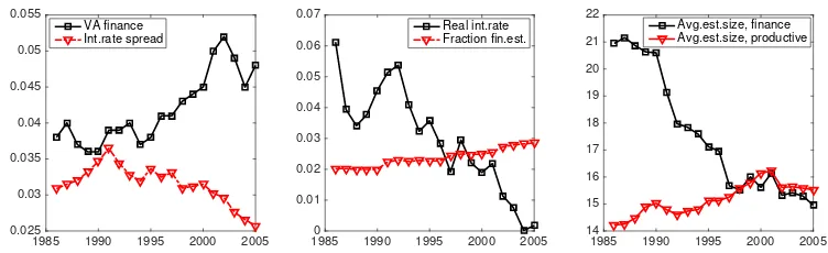
Figure 1: Characteristics of the financial intermediation sector, the US data
1985 1990 1995 2000 2005 0.025
0.03 0.035 0.04 0.045 0.05 0.055
VA finance Int.rate spread
19850 1990 1995 2000 2005 0.01
0.02 0.03 0.04 0.05 0.06 0.07
Real int.rate Fraction fin.est.
1985 1990 1995 2000 2005 14
15 16 17 18 19 20 21 22
Avg.est.size, finance Avg.est.size, productive
Note: The figure presents the US data on the financial sector value added and the interest-rate
spread (left graph); the real interest rate on savings and the fraction of financial sector establishments in total establishments (middle graph); the average establishment size, in terms of number of persons engaged, in the financial sector and all other sectors (right graph). Data sources are described in the Appendix.
added.
The rest of the paper is organized as follows. Section 2 briefly describes the trends
in the financial and production sectors’ characteristics using data from the US and
Tai-wan. Section 3 presents a model that incorporates the profit-maximizing producers and
financial intermediaries (bankers) in a general equilibrium framework with exogenous
sector-specific technological progress. Section 4 characterizes the properties of key
eco-nomic indicators derived from the model. Section 5 provides quantitative analysis of the
model: calibration to the U.S. economy, analysis of the model performance in replicating
the U.S. and Taiwanese data, and a number of counterfactual experiments evaluating
the importance of sector-specific technological progress and the financial intermediaries’
cost of capital for economic development in the US and Taiwan during the last three
decades. Section 6 concludes.
2
The Data and the Modeling Strategy
Figure 1 shows the time series of the key variables of interest: the financial sector
share of value added, the interest-rate spread, the average size (in terms of the number
of persons engaged) of the financial and production sector establishments, the fraction
of financial sector establishments, and the real interest rate on savings, using U.S. data
for 1986–2005. All the data and data sources are described in the Appendix.
Figure 2: Characteristics of the financial intermediation sector, Taiwanese data
1970 1980 1990 2000 2010
0.01 0.02 0.03 0.04 0.05 0.06 0.07 0.08
VA finance Int.rate spread
19700 1980 1990 2000 2010
0.02 0.04 0.06 0.08 0.1 0.12
Real int.rate Fraction fin.est.
19705 1980 1990 2000 2010
10 15 20 25 30 35
Avg.est.size, finance Avg.est.size, productive
Note: The figure presents the data for Taiwan on the financial sector value added and the
interest-rate spread (left graph); the real interest rate on savings and the fraction of financial sector establishments in total establishments (middle graph); the average establishment size, in terms of number of persons engaged, in the financial sector and all other sectors (right graph). Data sources are described in the Appendix.
five of these variables as an outcome of three possible causes: the unobserved
techno-logical progress in the production sector, the unobserved technotechno-logical progress in the
financial sector, and the observed changes in the real interest rate, a proxy of the
finan-cial intermediaries’ cost of capital. Thus, all key variables of interest (except for the real
interest rate) are endogenous variables, and the sector-specific technological progress
and the real interest rate are the only exogenous variables in the model.
In this respect, the model does not take into account the potential positive impact
of bank branch deregulation on technological progress in the US. The relaxation of
intrastate bank branch restrictions that started in the 1970s in the US could have
con-tributed to the financial development and to greater efficiency of the production sector
through easier access to loans and better monitoring (see Jayaratne and Strahan, 1996).
In addition, it could have led to growth in the fraction of financial sector establishments
in the total number of establishments, reported in Figure 1. However, in many U.S.
states the bank branch restrictions were lifted by 1986 (the starting year of the
analy-sis in this paper), and even if this deregulation served as a positive shock to financial
sector development, the dynamics of the size distribution of the bank branches
(finan-cial establishments in the model) and production establishments, the relative prices,
and the sector-specific value added can still be characterized as functions of exogenous
technological progress.
The other two trends characterizing the U.S. financial sector during the last three
sig-nificant decrease in the number of banks. The first of these trends is consistent with
the outcomes of the model, which predicts that technological progress leads to a larger
fraction of total capital being intermediated by the most efficient entrepreneurs. The
explanations of the potential drivers behind the second trend are not the purpose of this
paper. A number of studies (see, for example, Wheelock and Wilson, 2000; and Berger
et al., 1999 for a review of related literature) considered the quality of personnel
man-agement and asset manman-agement as the potential drivers behind numerous bank failures
and the mergers and acquisitions that led to the sharp decline in the number of U.S.
banks during the last three decades.
The model considered in this paper is based on interactions between production and
financial sector establishments where entrepreneurs in the production sector borrow
capital funds from financial sector entrepreneurs. The efficiency of each establishment
depends on the ability of the entrepreneur who manages the establishment
(correspond-ing to the bank branch in the financial sector). Thus, the model aims to explain the
trends characterizing U.S. bank branches rather than banks.
The US has been characterized by relatively stable economic growth rates during the
last three decades. To test the relevance of the model and to evaluate the importance of
sector-specific technological progress for economic development in an economy growing
at an unbalanced rate, I consider the data for Taiwan. Figure 2 reports the six key
variables of interest using the (available years within the period) 1971–2011 data for
Taiwan. Although not as transparent as for the US, the trends in the Taiwanese data
mostly resemble those for the US, except for the average size of the production sector
establishments which decreases for Taiwan.
Next, I describe the model, before taking it to the data and quantifying the impact
of financial development, production sector development, and the decline in the real
interest rate on the variables shown in Figures 1 and 2.
3
The Model
Consider an economy populated by two types of agents, “potential producers” and
“po-tential bankers,” with measure one of individuals of each type. The “po“po-tential
“potential bankers” are able to run a financial intermediary institution to supply loans
to entrepreneurs from the production sector and monitor their performance. Thus, the
agent’s type defines the sector in which the agent can perform entrepreneurial activity.
Depending on his ability, the agent can choose whether to become an entrepreneur in
his type-specific sector or to be hired as a worker. The distribution of agents’ abilities
within each type is time-invariant and characterized by cumulative distribution function
Fj(z) and probability density function fj(z), z ∈ [zj,z¯) in the production (j = e) and
financial (j = b) sectors, respectively. The productivity of a worker does not depend
on his entrepreneurial type; thus, the labor market is common for the production and
financial sectors.
All agents are born with zero assets. At the beginning of their lives, they decide
whether to become an entrepreneur of their type or to be hired in the labor market as
a worker. Those who decide to become entrepreneurs have a span of control to operate
a decreasing returns-to-scale technology and choose the optimal amounts of capital to
borrow and labor to hire, given expectations about the output that they can produce.
Each entrepreneurial project has a certain probability of failure, and the expected profits
depend on the entrepreneur’s ability. Each worker supplies one unit of labor in exchange
for the expected income given by the market wage. All agents receive their income and
decide on consumption and savings allocations at the end of the first period of their
lives. They retire and supply their savings to the active financial intermediaries at
the beginning of the second period of their lives. Finally, they consume their returned
savings and interest at the end of the second period of their lives and then die. Thus, each
agent lives for two periods, and in every period, there are two overlapping generations,
one working and one retired. The consumption and saving choices of an agent solve the
following utility maximization problem:
max
c1,h
u(c1) +βu(c2) (1)
s.t. :c1+h= Π, (2)
c2 = (1 +rb)h, (3)
where u(c) is the utility from consumption, u′(c) > 0, u′′(c) < 0; c
1 and c2 denote
of an agent (realized profits for entrepreneurs and realized wages for workers); β ∈(0,1)
is a discount factor;rb is the interest rate paid by financial intermediaries (bankers) for
savings; and h denotes savings. Assume that u(0) = u ' 0; that is, the agents whose
realized income is zero still enjoy some positive consumption (for example, by collecting
fruits from publicly available trees). Assume that u is sufficiently low so that all agents
prefer positive income and therefore, work either as entrepreneurs or as workers.
The problem of the individuals of each type, the role of abilities, and the markets
are described in more detail below.
3.1
The problem of a “potential producer”
Each individual of “potential producer” type decides whether to run a firm and produce
output in the form of final goods or to be hired as a worker in the labor market. The
decision is made based on the expected payoffs of these occupational choices.
The technology that a potential producer can operate has the following form:
ASe(z)1−q(kal1−a)q, (4)
where k and l are capital and labor hired by the entrepreneur; a ∈ (0,1) reflects the
importance of capital in production; q ∈ (0,1) is the span of control parameter (as in
Lucas, 1978); and ASe(z)1−q is the productivity level of a firm’s production process.
The productivity is the product of two components: the aggregate state of technology
in the production sectorAand an individual-specific productivity Se(z), which depends
on the entrepreneurial ability z, withS′
e(z)>0.
Given that entrepreneurs start life with zero assets, they have to borrow capital to
run their firms. The borrowing is complicated by two factors: the ultimate success of
the entrepreneur’s project is uncertain, and the entrepreneur can hide the final outcome
of his production project.
The production sector project is successful if output is produced according to
technol-ogy (4). The probability of success isˆπ; with probability1−πˆthe project is unsuccessful
and no output is produced.
The producer borrows capital from the financial intermediaries at the risk-adjusted
before he knows if his project is successful. Once the firm’s inputs are employed, a
random draw from a uniform distribution on [0,1] determines if the project is successful.
The entrepreneur can hide the successful realization of his project from the financial
intermediary with probability1−P, which depends on the level of financial development
in the economy and will be defined below. If the project is successful, the entrepreneur
produces final goods according to the technology (4), pays wages w/πˆ to employed
workers, and repays the loan conditional on successful monitoring by the intermediaries.
If the project is unsuccessful, the entrepreneur announces bankruptcy and does not
repay the loan to the financial intermediaries or the labor costs. For simplicity, the
liquidation value of the bankrupt firm is zero.
The maximization problem of the producer is the following:
max
k,l πASˆ e(z)
1−q(kal1−a)q−r
eP k−wl. (5)
For convenience, re-scale the probability of successful production project as follows:
ˆ
π =π1−q. The solution to problem (5) characterizes the optimal capital and labor inputs
as functions of producer’s ability, given wages, P, and interest rates:
l(z) =LeπSe(z), (6)
k(z) =hel(z), (7)
where
Le =
qA(1−a)1−aqaaq
w1−aq(reP)aq
1−1q
, (8)
he=
aw
(1−a)reP. (9)
The expected profits of the potential entrepreneur with ability z can be expressed
as follows:
EΠe(z) =LeπSe(z)w
1
q −1
1−a. (10)
with expected payoff EΠe(z) or to become a worker with expected payoff w. Given
that the expected profits are monotone increasing in ability, there is a threshold ability
z∗
e such that all potential producers with z ≥ ze∗ undertake an entrepreneurial project.
This threshold can be found from the following equation:
w=EΠe(ze∗). (11)
The potential producers with ability lower than z∗
e choose to become workers, so that
the total supply of labor from the group of potential producers is given by Rz∗e
ze fe(z)dz.
Given z∗
e,the total labor, L, and capital, K, demanded by the operating producers
are given by:
L=Le
Z z¯
z∗
e
πSe(z)fe(z)dz. (12)
K =heL. (13)
These quantities depend on wages, interest rates, prices and the set of active bankers,
which together with the set of active entrepreneurs (captured byz∗
e), are determined in
equilibrium.
Note, however, that the labor demand L can be rewritten as a function of z⋆
e only,
combining (8), (11), and (12), in particular,
L(z∗
e) =
Rz¯
z∗
e πSe(z)fe(z)dz
Se(z)
1−a
(1
q −1)π
. (14)
Therefore, the labor demand from the producers depend on wages and prices indirectly,
through their impact on the threshold z∗
e.
3.2
The problem of a “potential banker”
Each individual from the group of potential bankers decides whether to run a financial
intermediary institution or to be hired as a worker in the labor market. The decision
is made based on the expected payoffs of these occupational choices. If the potential
banker runs a financial intermediary institution, he can make profits by intermediating
d on the deposits market at a competitive deposit interest rate rˆb and sell loans to the
producers at the competitive expected loan interest rate re. The total cost of capital
for the financial intermediaries is rb = ˆrb+δ, where δ is the depreciation rate of capital
(similar to Greenwood et al., 2013). Parameter δ is constant throughout the model
and rb will be referred to as deposit interest rate. Each potential banker can operate a
common to the financial sector technology, which allows him to monitor borrowers to
reduce the probability 1−P of their hiding the successful realizations of projects.
Monitoring requires labor input, therefore the bankers also hire workers in the labor
market. The success of the monitoring depends positively on the banker’s ability, z,
through function Sb(z), with Sb′(z)>0, and labor input, x, and depends negatively on
the volume of intermediated funds,d. In particular (similar to Greenwood et al., 2010),
the probability of successful monitoring, P, is given by:
P = 1− 1
(T Sb(z)1−γxγ
d )ψ
, d
T xγ < Sb(z)
1−γ, ψ, γ ∈(0,1), (15)
where T > 0 represents the financial sector’s state of technology; γ reflects the
impor-tance of labor employed in the financial intermediation activities; and ψ is the span of
control in financial intermediation. Specification (15) implies that an increase in the
amount of capital intermediated requires more than a proportional increase in the labor
employed for the intemediation activities (because γ < 1), and decreases the
probabil-ity of successful monitoring (because ψ < 1). The inequality implies that the amount
of intermediated deposits adjusted for the technology-augmented labor effort must not
exceed certain level defined by the individual productivity of the banker to insure a
positive probability of successful monitoring. Assume that a(1− γ) +γ/q < 1 (this
assumption is not restrictive for a plausible range of parameters).
The maximization problem of the banker is the following:
max
d,x 1−
1
(T Sb(z)1−γxγ
d )ψ
!
red−rbd−wx, (16)
s.t. : d
T xγ < Sb(z)
1−γ. (17)
functions of the banker’s ability, given wages and interest rates:
x(z) =LbSb(z), (18)
d(z) =hbx(z), (19)
where
Lb =
γψT(re−rb)ψ1+1
wreψ1
(1 +ψ)ψ1+1
!1−1γ
, (20)
hb =
w(1 +ψ)
γψ(re−rb)
. (21)
Substituting the expressions for labor and deposits demand by a financial
intermedi-ary, obtain that the probability of success that each operating banker faces in equilibrium
depends only on the prices of capital:
P = ψre+rb
re(1 +ψ)
. (22)
For positive interest-rate spread, re−rb, P is bounded between zero and one.
Therefore, at optimum, the probability of successful monitoring is the same across all
active financial intermediaries. The intermediaries with less ability to monitor borrowers
will optimally choose to intermediate fewer funds.
The expected profits of the potential banker can be expressed as follows:
EΠb(z) = LbSb(z)w(
1
γ −1). (23)
Each potential banker decides whether to run an intermediary institution with
ex-pected payoff EΠb(z)or to become a worker with expected payoff w. There is a
thresh-old ability z∗
b such that all potential bankers with z ≥ zb∗ run a financial intermediary
institution. This threshold can be found from the equation:
w=EΠb(z∗b). (24)
The potential bankers with ability lower than z∗
the total supply of labor in the labor market from the group of potential bankers is
given by Rzb∗
zb fb(z)dz.
Given z∗
b, the total labor, X, and capital, D, demanded by the operating bankers
are given by:
X =Lb
Z ¯z
z⋆ b
Sb(z)f(z)dz, (25)
D=hbX. (26)
These quantities depend on wages, interest rates, prices and the set of active
en-trepreneurs. The labor demand from the financial intermediaries can be rewritten as a
function of z⋆
b only, combining (20), (24), and (25), in particular,
X(zb∗) =
R¯z
z∗
b Sb(z)fb(z)dz
Sb(z)
1
(1γ −1). (27)
Therefore, the labor demand from the bankers depend on wages and prices indirectly,
through their impact on the threshold z∗
b.
Two features of the financial sector are specific to this model and should be
high-lighted. First, the common probability of successful monitoring makes all financial
intermediaries identical from the point of view of both savers and borrowers. The set of
active financial intermediaries represents a homogeneous financial system that accepts
deposits and issues loans, performing monitoring along the way. Depositors can invest
in, and producers can borrow from, several financial intermediaries within a period.
In this sense, the model focuses on the determinants of the size of individual financial
establishments rather than on the determinants of the size of capital loans issued to
particular producers (differently from the related models with incentive compatibility
constraints imposed on borrowers, such as Greenwood et al., 2010 and 2013).
Second, the technology of the financial sector T includes the factors that make the
financial monitoring more efficient, and as formulated, is incomparable with the Solow
residual, commonly reported as an estimate of the sector technology. That is, T
repre-sents an unobserved technological progress. This unobserved process can potentially be
estimated given the observable variables, such as the interest-rate spread, as explained
3.3
The equilibrium
The focus of the analysis is on stationary equilibria. First, the market-clearing conditions
are presented. Second, a definition for a stationary equilibrium is given. Third, it is
shown that a stationary equilibrium for the model exists.
There are three markets in the model economy: a labor market, a market for deposits,
and a market for loans. The labor market is common for both sectors. The entrepreneurs
from the production and financial sectors demand labor according to functions L and
X, respectively. The agents who choose not to be entrepreneurs supply labor with the
total labor supply given by Rz¯
z∗
e fe(z)d(z) +
Rz¯
z∗
b fb(z)dz. The wage w adjusts to clear the labor market.
The market for loans arises because the borrowers (entrepreneurs from the
produc-tion sector) can shirk repaying their loans by falsely reporting their producproduc-tion projects
as unsuccessful. The financial intermediaries can monitor borrowers’ activities and
re-duce the probability of shirking, but the monitoring process is costly and requires some
labor input. Therefore, the interest rate on loans is greater than the deposit interest
rate. The supply of loans by the financial intermediaries is given byD, and the demand
for loans is given by K. The lending interest rate re adjusts to clear the loans market.
The market for deposits is characterized by the demand for deposits from the
finan-cial intermediaries, D, and the supply of deposits by the savers. In a closed economy,
savers are the retired agents, and the total supply of funds is a fraction of the total
profits generated in the previous period. The deposit interest rate rb adjusts to clear
the savings market. In an open economy, capital is supplied at interest rate rˆb which is
taken as given by the savers and the financial intermediaries (who face the capital cost
rb = ˆrb+δ). The data suggests that ˆrb was decreasing during 1986–2005 (see Figure 1),
and globalization of financial markets is considered to be the reason behind this decrease
(see Caballero et al., 2008). Therefore, further analysis focuses on the open economy
model as a more relevant framework.
The market-clearing conditions can be summarized in the following equations:
L(ze∗) +X(zb∗) =
Z ¯z
z∗
e
fe(z)d(z) +
Z z¯
z∗
b
fb(z)dz, (28)
These conditions define the prices re and w; rb is given in the open economy. More
formally, a competitive stationary equilibrium is defined as follows.
Definition: A competitive stationary equilibrium given rb, A, and T is described by
the thresholdsz∗
e, zb∗, allocations {k(z), l(z)}zz¯∗
e, {d(z), x(z)} ¯
z z∗
b, wagew, and interest rate
re, such that:
i) given w, re, and rb, all agents maximize their expected income by choosing their
occupation, and the thresholds z∗
e and zb∗ are determined, in accordance with (11)
and (24);
ii) given w, re, and rb, all producers and bankers choose capital and labor inputs to
maximize their expected profits; and
iii) the wage, w, and the lending interest rate, re, are determined so that the markets
for labor and loans clear, in accordance with (28)-(29).
The values of exogenous variables A, T, and rb determine the equilibrium prices, w
and re, as well as the set of active producers and bankers.
It is possible to show that given any positive values of these variables, there exists a
unique equilibrium for the model economy.
Proposition 1: For any positive values of A,T, andrb, there is a unique stationary
equilibrium for the model economy.
(All proofs are in the Appendix.)
The impact of the interest raterb and the technological progress, in either the
finan-cial or production sector, on the economy can now be characterized.
4
Characterization
The aim is to analyze the impact of sector-specific technological progress and the real
interest rate on macroeconomic indicators, such as the economic output, the capital
to output ratio, value added by sector, sector-specific distribution of establishments
by size in terms of employment, and quantity of establishments by sector. First, the
Second, the pattern of responses of each of these indicators to a change in A, T, or rb
is established. Then, in the next section the model predictions are compared to the
patterns in the data, and the model-implied trends of A and T in particular countries
are discussed.
Given prices and thresholds z∗
e and zb∗, the aggregate macroeconomic indicators can
be computed as follows.
The interest-rate spread,s, can be derived from the capital market clearing condition:
s =re−rb =
(1−a)(1 +ψ)X(z∗
b)
aγψL(z∗
e)−(1−a)ψX(zb∗)
rb. (30)
The expected total output, Y, is given by the sum of the total expected profits (of
entrepreneurs, workers, and savers) or equivalently, by the total expected output in the
final goods sector, as follows:
Y =
Z z¯
z⋆ e
A(πSe(z))1−q(kal1−a)qfe(z)dz =haqe LqeA
Z z¯
z⋆ e
πSe(z)fe(z)dz. (31)
The economy’s output is proportional to the production sector technology, A, the
quantity of labor hired by the production sector, and the probability of successful
pro-duction, π, and negatively depends on the producer’s costs of labor, w, and capital,
reP.
The total capital to output ratio, from (13) and (31), is given by the following
expression:
K Y =
aq reP
= aq(1 +ψ)
ψs+ (1 +ψ)rb
= aq(1 +ψ)
ψre+rb
. (32)
The model predicts that the capital-output ratio increases with a decrease in the
interest-rate spread, s, or the deposit rate,rb.
The financial sector value added is given by the total profits of the financial
in-termediaries plus the labor costs or by the financial sector output minus the financial
intermediaries’ cost of capital. The financial sector value added as a share of the output
is as follows:
V Ab = (reP −rb)
K Y =
ψaqs
ψs+ (1 +ψ)rb
= ψaq(re−rb)
ψre+rb
. (33)
intermediaries’ cost of capital,rb. The share of financial sector value added is decreasing
inrb, because it becomes more costly to produce loans as the deposit rate increases and
therefore, the supply of loans decreases. The share of financial sector value added
is increasing in s and re, because it is more profitable to supply loans as their price
increases, other things equal.
Similarly, the production sector value added is given by the total profits of the
producers plus the labor costs or by the production sector output minus the producers’
cost of capital input. The production sector value added as a share of output simplifies
as follows:
V Ae=
Y −reP K
Y = 1−aq. (34)
It is constant in the model economy, equal to one minus the share of capital in the
production. A fraction aq of value added is generated by the financial intermediation of
capital, which contributesV Ab, and by the savers, who invest their capital with financial
intermediaries and contribute rbK to the total value added.
In addition to these standard indicators of economic performance, the measures of
establishment size, quantity, and size distribution by sector can be computed in model
terms, given the values ofA,T,rb, and parameters. Along with economic output
indica-tors, these measures can be used to evaluate the impact of sector-specific technological
progress on the economy.
The quantities of firms operating in the production and financial sectors, Qeand Qb,
respectively, are given by:
Qe=
Z z¯
z∗
e
fe(z)dz, (35)
Qb =
Z z¯
z∗
b
fb(z)dz. (36)
The sector-specific average size of the establishment can be computed as the ratio
of the total sector-specific labor demand to the quantity of establishments in a given
LQe =
L(z∗
e)
Rz¯
z∗
efe(z)dz
, (37)
LQb =
X(z∗
b)
Rz¯
z∗
b fb(z)dz
, (38)
whereLQe and LQb stand for the average size of the establishment in terms of
employ-ment in the production and financial sectors, respectively.
The establishment size distribution in a given sector can be characterized by the share
of employment in the smallestN percent of establishments in that sector, computed as
follows:
LQe,N =
RzeN
z∗
e Se(z)fe(z)dz
Rz¯
z∗
e Se(z)fe(z)dz
, where zeN solves: N = Fe(z
N
e )−Fe(z∗e)
1−Fe(ze∗)
; (39)
LQb,N =
RzNb
z∗
b Sb(z)fb(z)dz
Rz¯
z∗
b Sb(z)fb(z)dz
, where zbN solves: N = Fb(z
N
b )−Fb(zb∗)
1−Fb(z∗b)
, (40)
for different Ns.
The economy growing at an exogenous growth rate determined by the relative growth
rates of A and T and given rb, can now be characterized.
Proposition 2: Let T grow at rate g, A grow at rate (1 +g)1−aq −1, and r b be
constant. There exists a balanced growth path where the wages, output, demand for loans,
and demand for deposits all grow at rate g. The thresholds z∗
e and z∗b, the quantity and
the average size of establishments in the production and financial sectors, labor demand
and supply, and the lending interest rate remain constant.
This result is similar to the conclusion of Greenwood et al. (2010) that balanced
development of the production and financial sectors does not make the financial sector
more efficient. The probability of catching the firm that misrepresents its earnings is
constant over time. The quantity of active establishments in both sectors does not
change over time.
For a constant rb, unbalanced growth occurs whenever technology in either sector
tech-nological progress in the financial sector makes it more efficient in comparison to the
production sector (P increases). The relative cost of monitoring producers drops,
lead-ing to higher competition for deposits, lower interest rates for loans, and crowdlead-ing out of
the least efficient financial intermediaries. At the same time, the greater supply and the
lower price of funds make borrowing affordable for less efficient producers. Therefore,
technological progress in the financial sector leads to worsening of the pool of borrowers
from the production sector.
The opposite occurs when the production sector’s technology grows relatively faster
than the financial sector’s technology: The demand for loans increases, increasing their
price and crowding out the least efficient producers. High demand for loans makes
financial intermediation profitable for less efficient financial intermediaries and reduces
the relative efficiency of the financial system.
Proposition 3: (a) Let A grow at rate (1 +g)1−aq−1, T grow at rate g′ <(>) g,
and rb be constant. The threshold ze∗, the financial sector value added, and the
interest-rate spread increase (decrease) over time; the thresholdzb∗ and the capital-to-output ratio
decrease (increase) over time; output grows at a rate lower (greater) than g.
(b) Let A/T grow at rate (1 + g)−aq − 1, and rb decrease (increase) over time. The
threshold z∗
e, the financial sector value added, and the capital-to-output ratio increase
(decrease) over time; the threshold z∗
b and the interest-rate spread decrease (increase)
over time; output grows at a rate greater (lower) than g.
A decrease in the exogenously given rb and a decrease in the financial sector
technol-ogy T affect the capital-output ratio and the interest-rate spread in opposite directions
while having a similar impact on the set of active entrepreneurs in each sector and the
financial sector value added. In both cases, the financial sector becomes relatively less
efficient. A drop in T implies that the financial sector technology is relatively low,
leading to greater producer cost of capital and slower output growth. A drop in rb
implies lower financial intermediaries’ cost of capital and leads to the supply of capital
for producers at lower prices, accelerating output growth.
Proposition 3 establishes how the quantity of establishments in a particular sector
responds to the changes in sector-specific technologies or in the deposit interest rate. An
least efficient producers (those with lower z) out of business. As a result, the quantity
of establishments decreases. The opposite happens in the sector which experiences a
relative decrease in its aggregate sector-specific technology. The impact on the average
establishment size, LQe and LQb, is uncertain in general and depends on the functions
Se and fe (Sb and fb). In the quantitative analysis, these functions are selected to
replicate the observed patterns of the average establishment size and establishment size
distributions in the US.
The next section uses observable data, such as the real interest rates on savings and
the interest-rate spread, the total output, the financial sector share of output, and the
establishment size distributions to quantitatively characterize the importance of changes
in A,T, and rb for the economy.
5
Quantitative Analysis
The aim of this section is to evaluate the model performance in replicating the data and
to quantify the importance of changes inA,T, andrb for economic development. First,
the values of the model parameters are chosen to fit a number of empirical facts from the
U.S. economy. Second, the values of macroeconomic indicators predicted by the model
are compared to their counterparts in data from the US and Taiwan. Third, the impact
of sector-specific technological progress or a decrease in the financial intermediaries’ cost
of capital on economic output is analyzed.
For quantitative analysis, the functions Se andSb, which describe individual-specific
productivity in the production and financial sectors, and the abilities distribution
func-tions, fe and fb, must be specified. Let the abilities of each type of agent follow Pareto
distribution with the following parameters:
fe(z) = vezveez−ve−1, z∈[ze,∞), ve>1; (41)
fb(z) =vbzvbbz−vb−1, z ∈[zb,∞), vb >1. (42)
The corresponding cumulative distributions are Fe(z) = 1−zveez−ve and Fb(z) = 1−
zvb
b z−vb, for the production and financial sectors, respectively.
z. Consider the following functions:
Se(z) = ce,0+ce,1zse, ce,0, ce,1 >0, se∈(0, ve); (43)
Sb(z) =cb,0+cb,1zsb, cb,0, cb,1 >0, sb ∈(0, vb). (44)
The restrictions on the coefficientsce,0 andcb,0 imply that the average establishment
size in the production and financial sectors is increasing in the thresholds z∗
e and zb∗,
respectively. The restrictions onseandsb are necessary to generate finite labor demand.
5.1
Calibration
The model economy is fully characterized by five variables: z∗
e,z∗b,A,T, and rb. Onlyrb
is observable and can be taken directly from the data. The properties of z∗
e, zb∗,A, and
T can be gauged by analyzing the observed characteristics of the variables influenced
by these unobservables. This is done as follows.
Parameter δ is assigned the standard value used in the literature, 0.05. Parameter
a measures the importance of capital in production and is determined together with
parameterqso that the aggregate capital shareaq is equal to0.30. Parameterψgoverns
the share of the financial sector value added, V Ab defined by (33). I use ψ = 0.97, in
line with Greenwood et al. (2013); the values of ψ in the range (0.9–0.99) deliver the
model-predicted level of financial sector value added close to that observed in the data.
Given the model parameters, PARAM={{cj,0,cj,0,vj,sj,zj}j∈{e,b},δ,a,q,γ,ψ,π}, and
given the values of the exogenous variables, EXVARS={A,T,rb}, the thresholdsz∗e and
z∗
b fully characterize the sector-specific average establishment sizes, LQe and LQb, and
establishment distributions by employment size (which can be described by the share of
employment in the smallestN percent of establishments, for differentNs, using (39) and
(40)). Therefore, the empirically relevant thresholdsz∗
e andzb∗ can be found by choosing
the model parameters PARAM\{δ, a, ψ}, given the exogenous variables EXVARS, to
minimize the distance between the model-predicted and empirical values of the average
establishment sizes and establishment size distributions in the production and financial
sectors. Following Greenwood et al. (2013), I consider the share of employment in the
smallest 60, 75, 87, 95, 98, 99.3, and 99.7 percent of establishments to describe the
The levels of the exogenous sector-specific technologies,AandT, have a direct impact
on the production and financial sector output and determine relative prices, including
the interest-rate spread. In particular, given rb and the parameters, the equilibrium
of the economy can be considered as providing the mapping between the aggregate
level of output, Y, and the interest-rate spread, s, on the one hand, and the state of
technology in the production and financial sectors, A and T, on the other.
Repre-sent this mapping by (Y,s)=M(PARAM,EXVARS). This mapping can be used to make
an inference about (A, T), given an observation on (Y, s), by using the relationship
(A,T)=M−1(PARAM,Y,s,r
b), as in Greenwood et al. (2013).
The model is calibrated to the U.S. economy. As a measure of the cost of capital ˆrb,
I use the estimate of the global real interest rate from Caballero et al. (2008), computed
as the weighted average of the interest rates on 3-month Treasury bills adjusted for
inflation in the next quarter among the leading economies. This interest rate is highly
correlated with the estimates of the U.S. real interest rate and with the estimates of
the global real interest rate by King and Low (2014), and it is inconsequential which
one is used in the estimation. What matters is the downward trend characterizing the
U.S. and the global real interest rates during 1986–2005. The deposit rate rb is then
computed as ˆrb +δ.
Detailed sectoral data on the distribution of establishments by employment size is
available on an annual basis starting from 1986 (at the U.S. Census Bureau, County
Busi-ness Patterns). I consider the data for sectors with SIC codes 6000 and 6100 (NAICS
code 522///) which correspond to financial intermediation as a counterpart of the
finan-cial sector in the model and data on all other sectors minus finanfinan-cial intermediation as a
counterpart of the production sector in the model. During the period 1986–2005, there
are no significant changes in the overall establishment size distributions. Therefore, I
use the 1986 year data for the calibration targets. At the same time, during the period
1986–2005, the average size of the financial sector establishments decreases, and the
average size of the production sector establishments increases. To achieve significant
responses of the establishment size to changes in the thresholds z∗
e and zb∗, PARAM are
chosen so that the elasticity of the average production (financial) sector establishment
size with respect to threshold z∗
To summarize, the calibration procedure is as follows:
(a) given deposit interest rate rb, the values of parameters δ and ψ, and a guess for
the remaining PARAM:
(a.1) the values of z∗
e,zb∗, w, and re are found from equations (28), (29), (11), and
(24) jointly with
(a.2) the values of A and T such that the model-generated output, Y, and the
model-generated interest rate spread, re−rb, are equal to the U.S. real GDP
per capita (in thousands) and the U.S. interest-rate spread in 1986; and
jointly with
(a.3) the values of parameters γ, q, and a such that the financial and
produc-tion sectors model-generated average establishment sizes are equal to their
counterparts in 1986 U.S. data and the aggregate capital share is0.30;
(b) step (a) is repeated until the sum of the squares of the differences between the
model-generated and the 1986 observed shares of employment in the smallest 60,
75, 87, 95, 98, 99.3, and 99.7 percent of establishments together with the inverses
of the model-implied elasticities of the average establishment sizes with respect
to thresholds z∗
e and zb∗, for the production and financial sectors, respectively, is
minimized, subject to the following constraints: se < ve, sb < vb, ve, vb > 1,
ce,1, cb,1 >0, 0< π <1.
Table 1 reports the parameter values. The two parameters that are standard in the
literature, the importance of capital in production, a = 0.365, and the span-of-control
in the production sector, q = 0.823, calibrated to match the aggregate share of capital
and the production sector average establishment size, are within the range of the values
used in the literature (0.28–0.40 and 0.8–1, respectively; see Greenwood et al., 2013
and Guner et al., 2008). The calibrated probability of successful production projects is
relatively high, π = 0.873, suggesting that more than 80 percent of the establishments
in the final good sector generate positive output.
Figure 3 presents the cumulative share of employment in the production and financial
sector establishments in the 1986 U.S. data and in the model. The model overestimates
establishment size distributions, respectively, while fitting the middle relatively well.
This is because there is a trade-off between the magnitude of the establishment size
elasticities, LQe
dLQe dz∗
e z
∗
e and
LQb dLQb
dz∗
b z
∗
b
and a good fit of the establishment size distributions. If
the establishment size elasticities are excluded from the minimization function, then
the model-generated distributions are closer to their empirical counterparts, but the
implied elasticities are zero, which contradicts the data. The experiments suggest that
more complex distributions of abilities or individual technologies functions Se and Sb
[image:26.595.115.466.284.533.2]have little impact on calibration results.
Table 1: Parameter Values
Parameter Value
Depreciation rate,δ 0.050
Probability of successful production, π 0.873 Importance of capital in production, a 0.365
Importance of labor in finance,γ 0.864
Span of control in production,q 0.823
Span of control in finance,ψ 0.970
Shape parameter, abilities distribution in production,ve 1.371
Shape parameter, abilities distribution in finance,vb 1.726
Scale parameter, abilities distribution in production,ze 1.036 Scale parameter, abilities distribution in finance, zb 0.734 Constant, individual efficiency in production,ce,0 5.805 Constant, individual efficiency in finance, cb,0 273.322 Scale parameter, individual efficiency in production,ce,1 2.264 Scale parameter, individual efficiency in finance, cb,1 2.928 Shape parameter, individual efficiency in production,se 1.158
Shape parameter, individual efficiency in finance, sb 1.478
Note: The table reports the values of the parameters obtained from the calibration of the model to
the U.S. data.
5.2
Simulations
I simulate the model for the US (on an annual basis, during 1986–2005) and for Taiwan
(every fifth year, during 1971–2011) because the necessary data (or plausible proxies)
for these countries and time periods are available. For each country, given the values of
the parameters reported in Table 1, I simulate the model along the equilibrium growth
path at which the model-generated output replicates the annual country’s real GDP per
capita, the model-generated rate spread replicates the country’s annual
Figure 3: Establishment size distribution, 1986 US data and model
0 0.2 0.4 0.6 0.8 1
Establishments, percentile
0 0.2 0.4 0.6 0.8 1
Employment, cumulative share
Productive Sector
Data Model
0 0.2 0.4 0.6 0.8 1
Establishments, percentile
0 0.2 0.4 0.6 0.8 1
Employment, cumulative share
Financial Sector
Note: The figure presents the cumulative share of employment in the smallest N percent of
establishments in the 1986 US data (black line with triangles for data points) and in the model (red line with stars for data points). The left and right graphs report the values for the production and financial sectors, respectively. Data sources are described in the Appendix.
interest rate plus depreciationδ. That is, I repeat steps (a.1) and (a.2) of the calibration
procedure for every year from 1986 to 2005 for the US or every fifth year from 1971 to
2011 for Taiwan, using the values of PARAM from Table 1.
The following key model-generated variables are functions of unobservable A and T
(or equivalently, of observable Y and re −rb) and can be used to evaluate the model
performance: the financial sector value added (the production sector value added is
constant given by (34)), the sector-specific employment size, and the quantity of
estab-lishments in each sector. The performance of the model in replicating each variable for
the US and Taiwan is discussed next.
5.2.1 Results for the US
Table 2 summarizes the U.S. data for the first and last years of the time period
consid-ered, 1986 and 2005, and the values of the corresponding variables in the model. Figure
4 plots the time series of three key model-generated variables, the financial sector share
of value added, the average establishment size in the financial sector, and the fraction of
financial sector establishments, and their empirical counterparts for the US. The model
captures (with different degrees of quantitative success) the increase in the financial
sector value added during 1986–2005 and the trends in the sector-specific establishment
characteristics: an increase in the average size of the production sector establishments,
a decrease in the average size of the financial sector establishments, and an increase in
The model-predicted share of financial sector value added, which can be computed
independently of any other predictions of the model using the observable values of rb
and s, is very close to its empirical counterpart, and the two variables move together
over time (see Figure 4, left panel). The capital-to-output ratio in model terms is linked
to the financial sector value added and can be computed from the data onrb and sand
the given parameters a, q, and ψ. The model-generated values are close in magnitude
to their empirical counterparts, although the model predicts an increase in the
capital-to-output ratio, while in the data the ratio is relatively stable over time.
The model-generated values for the thresholds of abilities characterizing active
en-trepreneurs, z∗
e and zb∗, and for the technology levels, A and T, can be used to make
inferences about the potential drivers behind the trends observed in Figure 4.
Accord-ing to the model, given the trends in the U.S. output and the interest-rate spread, the
minimum (and average) entrepreneurial efficiency in the production sector increased,
while the minimum (and average) entrepreneurial efficiency in the financial sector
de-creased during 1986–2005. Thus, the average financial sector entrepreneur became less
efficient over time, and the average production sector entrepreneur became more
effi-cient over time; as a consequence, the fraction of the financial sector establishments
increased. This could happen for either or both of the following reasons: (1) because
the financial sector technology grew at a rate that was lower than the rate necessary
to maintain the constant relative efficiency of the production and financial sector and
(2) because the financial intermediaries’ cost of capital, the interest rate on savings,
decreased. The growth rates of the production and financial technologies over 1986–
2005 are 0.0050 and 0.0107, respectively (these values can be obtained from Table 2
using formula gZ = (Z2005/Z1986)1/(2005−1986) −1, where Z = T, A). From Proposition
3, for a balanced growth path along which T grows at rate g = 0.0107, A should grow
at rate (1 +g)1−aq −1 = 0.0075. Thus, the financial sector technology grew at a rate
greater than the rate required for the balanced growth path. According to the model,
this should lead to an increase in the relative efficiency of the financial sector and to the
growth of the total output at a rate greater than g.
However, the real interest rate decreased during 1986–2005. The fact that the relative
Table 2: Results: the US data and the model
1986 2005
Data Model Data Model
Output,Y 33.400 33.400 49.583 49.583
Int. rate spread,s=re−rb 0.031 0.031 0.026 0.026
Finance value added, V Ab 0.038 0.036 0.048 0.059
Capital-to-output,K/Y 3.213 2.373 3.017 4.658
Avg. est. size production, LQe 14.223 14.223 15.526 14.346
Avg. est. size finance,LQb 20.949 20.949 14.957 15.837
Fraction of finance est., 1−Fb(zb∗)
2−Fb(z∗e)−Fb(zb∗) 0.020 0.039 0.029 0.081
Min. entrepr.efficiency prod.,Se(ze∗) 19.552 20.072
Min. entrepr.efficiency fin.,Sb(z∗b) 445.103 364.742
Production technology,A 4.423 4.860
Finance technology, T 4102.9 5019.9
Note: The table reports the values of the variables observed in the US in 1986 and 2005, in columns
“Data,” and the corresponding model-generated values, in columns “Model.” The model-generated values are obtained from the simulations along the equilibrium growth path at which the
model-generated output replicates the annual U.S. real GDP per capita, the model-generated
interest-rate spread replicates the U.S. interest-rate spread, and the interest raterb in the model is
equal to global real interest rate plus depreciationδ. The last four rows report the model-generated
variables which do not have observable counterparts in the data.
financial sector entrepreneur’s efficiency and an increase in the financial sector share of
value added) implies that the impact of the relative improvement in the financial sector
technology was overturned by the decrease in the real interest rate. This led to a decline
in the probability of successful monitoring of borrowers,P, defined in model terms, from
0.89 to 0.83 between 1986 and 2005.
At the same time, according to the model, the decline in the real interest rate
contributes to the total output growth. Therefore, the financial sector technology growth
rate 0.0107 combined with the observed decline in the real interest rate is consistent with
the output growth rate 0.021, as observed in the US during 1986–2005.
5.3
Results for Taiwan
Taiwan is one of the few countries for which some data on the establishment size
distri-bution by sector is available (all data sources are in the Appendix). In addition, Taiwan
experienced rapid economic growth in the last three decades and a sharp decline in
the interest-rate spread, from 0.0744 in 1971 to 0.0196 in 2011. Therefore, I check the
model performance in explaining the patterns of the key variables using Taiwanese data
Figure 4: Characteristics of the financial sector, the U.S. data and the model
1985 1990 1995 2000 2005
0.035 0.04 0.045 0.05 0.055 0.06 0.065 Value added Data Model
1985 1990 1995 2000 2005
14 15 16 17 18 19 20 21 22
Average employment size
1985 1990 1995 2000 2005
0.01 0.02 0.03 0.04 0.05 0.06 0.07 0.08 0.09
Share of establishments
Note: The figure presents the U.S. data (black lines with triangles for available data points) and the
[image:30.595.103.503.305.428.2]model-generated data (red lines with stars) for financial intermediation sector. The left graph reports the share of value added; the middle graph reports the average establishment size measured by the number of persons engaged; the right panel presents the share of financial establishments in total establishments. Data sources are described in the Appendix.
Figure 5: Characteristics of the financial sector, Taiwanese data and the model
1980 1990 2000 2010 0.025 0.03 0.035 0.04 0.045 0.05 0.055 0.06 Value added Data Model
1970 1980 1990 2000 2010 10 15 20 25 30 35
Average employment size
19700 1980 1990 2000 2010 0.02 0.04 0.06 0.08 0.1 0.12 0.14
Share of establishments
Note: The figure presents the Taiwanese data (black lines with triangles for available data points)
and the model-generated data (red lines with stars) for financial sector. The left graph reports the share of value added; the middle graph reports the average establishment size measured by the number of persons engaged; the right panel presents the share of financial establishments in total establishments. Data sources are described in the Appendix.
fifth year starting from 1971 until 2011. The data on financial sector value added is
available from 1981. For consistency with the analysis for the US, I consider 2006 the
final year. As an estimate of the real interest rate on savings, I consider the Taiwanese
annual deposit interest rate adjusted for inflation. That is because although there is no
significant difference between the U.S. real interest rate and the global real interest rate,
the Taiwanese real interest rate is significantly higher than the global real interest rate.
Table 3 reports the data and model values for 1981 and 2006. Figure 5 shows the
time series for three key variables in the data and corresponding variables generated by
the model: the financial sector share of value added, the average establishment size in
Table 3: Results: Taiwanese data and the model
1981 2006
Data Model Data Model
Output,Y 10.132 10.132 35.958 35.958
Int. rate spread,s=re−rb 0.044 0.044 0.024 0.024
Finance value added, V Ab 0.031 0.037 0.046 0.045
Capital-to-output,K/Y 1.436 1.713 2.479 3.859
Avg. est. size production, LQe 8.300 14.230 6.300 14.273
Avg. est. size finance,LQb 35.000 20.580 18.300 18.419
Fraction of finance est., 1−Fb(zb∗)
2−Fb(z∗e)−Fb(zb∗) 0.006 0.041 0.018 0.055
Min. entrepr.efficiency prod.,Se(ze∗) 19.579 19.761
Min. entrepr.efficiency fin.,Sb(z∗b) 438.139 401.342
Production technology,A 2.118 4.058
Finance technology, T 847.996 4776.4
Note: The table reports the values of the variables observed in Taiwan in 1981 and 2006, in columns
“Data,” and the corresponding model-generated values, in columns “Model.” The model-generated values are obtained from the simulations along the equilibrium growth path at which the
model-generated output replicates the annual Taiwanese real GDP per capita, the model-generated
interest-rate spread replicates the Taiwanese interest-rate spread, and the interest raterb in the model
is equal to Taiwanese real interest rate plus depreciationδ. The last four rows report the
model-generated variables which do not have observable counterparts in the data.
The model-specific variables measuring the sector-specific entrepreneur’s efficiency
suggest that the Taiwanese financial sector became relatively less efficient during the
considered time period. The computations similar to those performed for the US suggest
that the production sector technology grew at a rate of 0.0263, while the financial sector
technology grew at a rate of 0.0716, which is greater than the balanced growth path
rate given the growth rate of A. At the same time, similar to the US, the financial
intermediaries’ cost of capital declined in Taiwan. This decline in the real interest rate
overturned the impact of the financial sector technology growth on the relative efficiency
of the financial sector.
The observed trends in the Taiwanese sector-specific establishment size
character-istics are non-linear (see Figure 5). There was an increase in the average size of the
financial sector establishments in 1986 compared with previous years, followed by a
de-cline until 2011. The model replicates some of the dynamics (none of the Taiwanese data
was used as the calibration target) on the average employment size and the fraction of
the financial establishments. The model also predicts the share of financial sector value