Blow-Up and Attractor of Solution for Problems of
Nonlinear Schrodinger Equations
Ning Chen*, Jiqian Chen
School of Science, Southwest University of Science and Technology, Mianyang, China Email: *[email protected]
Received September 18, 2012; revised October 18, 2012; accepted October 26, 2012
ABSTRACT
In this paper, the authors study the blow-up of solution for a class of nonlinear Schrodinger equation for some initial boundary problem. On the other hand, the authors give out some analyses and that new conclusion by Eigen-function method. In last section, the authors check the nonlinear parameter for light rule power by using of parameter method to get ground state and excite state correspond case, and discuss the global attractor of some fraction order case, and com- bine numerical test. To illustrate this physics meaning in dimension d = 1, 2 case. So, by numerable solution to give out these wave expression.
Keywords: Nonlinear Schrodinger Equation; Eigen-Function Method; Fractional Order; Blow-Up; Glabal Attractor
1. Introduction
The quantum mechanics theory and application in more field in nature science. The non-linear Schrodinger equa- tion is the basic equation in nonlinear science and widely applied in natural science such as the physics, chemistry, biology, communication and nonlinear optics etc. (See [1-9]) We study this equation to extend them are with important meaning (See[10-12]).
As we all know, the nonlinear Schrodinger equation be description quantum state of microcosmic grain by wave, it is variable for dependent time, and that is most essen- tial equation, which position and action similarly Newton equation in position and action classics mechanics, it is apply to field as optics, plasma physics, laser gather, co- hesions etc, particular on that action of power and trap, search analytical solution for Schrodinger equation is also difficult, and more so difficult for complicated power.
Now, we may extend some results in [4] by using Ei- gen-function method in through paper.
As we all know the solution of initial problem for Schrodinger equation bellow
2
i , , ,
,0 ,
n t
n
u a u f x t x R t
u x x x R
0,
(1.1)
Assume that real part and imaginary part of
x ,f x t, ,
are real analytical function for n,
xR then this solu-tion of the problem may expresses in form:
2 0 0
i ,
!
, d . k
k k k
t k k
x a
u x t t x
k
t f x
2. Several Theorems
In this section, we consider the blow-up of solutions to the mixed problems for higher-order nonlinear Schrod- inger equation with as bellow.
It is well known the higher order equation:
,i k , 0,
t
u u f u t x
where
22 2 1
, ,
n
i xi
,etc.that with new results for higher-order case. Now, we consider the blow-up of solutions to the mixed problems for six-order general Schrodinger equation to extend some results [4] that as bellow form:
3
2
i , 0, ,
0, , ,
, ,
t
u u f u t x
u x x x
t x u t x u t
0, 0.
(2.1)
Assume that
0,
4k 1,
6
,f f c x H
x
not identical zero.
Where f holds complex value function with self-
x.
variable for comple
x is also complex valueTheorem 2.1. Suppose that nonlinear term
2 2 0, , 1 n
t x R R
f of pro-
blem (2.1) satisfy C0,
0,
4k 1,
6
,f c x H
f
and
x) must be
not identical zero then the classical solution of (2.1 for blow-up in finite time in
Proof. Let
1 0, ; 6 .
C T H
2d d ,
J t
u x uu x
(2.2) Then
3 3
d
i d
t i
d ,
u u uu x
u u u u x u f u uf u x
(2.3)By the first Green’s formula, we have
J t
2 1
3 2 2
1
d
d d d
i
i i
x i
n
x x
i
u x
u u x u u s u u x
Substituting it into (2.3), then
3 d 2 d
i
n x
u u x u u s u
3 3
d
d ,
u u
J t i
u u su f u uf u x
We may assume
t x, 0,then we have2 u
u u u u u u
2
0.
u
Obviously, from u f u
uf u
2u f u
, and
4 1.
k
f u c u Therefore, we have
4d
k
d 2
J t
u x.By Schwartz inequality:
u f u uf u x c
2
2d 1d
u x x
41
d , here d 0.
u x c x
So,
24 2
1
d 1 d
u x c u x
.Inductively, we have
2
6 31 d
c
u x etc.,12
d 1
u x
4
2
21
d 1 d 0.
k k
k
u x c u x
Then J t
increasing function similar in [4 from ]
2
4 2
1 1
2 d 2 d
2 1
2 0,
k
k k
k k
J t
c c J t
and then there exists
c c u x c c u x
such that
0lim ,
t T J t
0 ,
T
that is
0
2 lim dx .
t T
uSo, we complete the proof of this Theorem 2.1. (As positive integer k1,we get i 3.1 in
[4
r equ
t is theorem ])
onside
Remark. Then we c r that important case is al-ways for the Schrodinge ation may as bellow form
0 :
i 2 2t
c u u c u u.
Now, we shall consider also in this similar case:
2 3
2
i ,
t
u u c u u
0, , ,
, , 0, 0.
u x x x
t x u t x u t
(2.4)
Therefore, we shall obtain the following theorem. Theorem 2.2. Suppose that non-linear term f of
problem (2.1) satisfy
c0
,
4 10, k ,
f f c
and
6
, 0, 2 2 0, ,
1 n,x H x t x R R
e classical solution of (2.4) must be for blow-up in finite time in
then th
1 0, ; 6
C T H (as positive k1, then
it is theorem 3.2 in [4]).
Proof. Since f u
c u2u c,
0
satisfies
2 40
f c
k
c
,
then
4k 1.f c
Thus, from theorem 2.1, we complete the proof of m 2.2.
theore
Now, we shall give out the following theorem form. Here, we shall consider the problem:
2 3
i , 0, ,
t
u u F u u t x
2
0, , ,
, , 0, 0.
u x x x
t x u t x u t
(2.5)
blem (2.5) satisfy
c0
, F
c4k3,
x 0,and
,
6
, 2 2 0, ,
1 nx H t x
R R
th bl
(As positive i then it is theorem 3.2 in [4])
oof. Since
en the classical solution of (2.5) must be for ow-up in finite time in 1
C 0, ;T H6
. nteger k1,Pr f u
F u
2 u c,
0
, we have that
2 4 1,
k
f F c
and
2 4k0.
f c c
eorem 2.1, we complet theorem 2.3. (As it is theorem 3.3 in [4])
Now, we may consider the following problem:
Thus, from th e the proof of
1, k
2 3
i e 1 , 0, ,
0, , ,
p s t
u u k u t x
u x x x
(2.6)
wh
Theorem 2.4. that and
then the solution of (2. w-up
me in 2
, , 0, 0.
t x u t x u t
ere constant k0,p0.
Assume
x H6
, 6) must be for blo
x 0,
in finite ti 1
0, ; 6
C T H .
Proof. From
2 2 1 2 2
e 1
2!
p u
p u p u
,
then
ep u2 1
f u K u satisfy f
0, and
4kf 1.
It holds the condition of theorem 2.1, then by theorem 2.1 that we know the solution of problem (2. ) must be blow-up in finite time. Therefore, we complete the proof
orem 2.4.
3. Main Results
Wermore, we will consider eight-order nonlinear Schrodinger equation. In first, stating that lemma 3.1.
Lemma 3.1. This Eigen-value problem (see [4])
kp
6
of the
e consider the initial boundary value of some higher order nonlinear Schrodinger equation. By using of eigen- function method, we can get new results bellow.
Let
t, x
Du u D u
, 1, 2 ,
,n
t x x x
u u u u
11 2
, , , , 1, 2, , ,
, , , .
i i x i
i
n
tx x x x x x
x x x x
Du u u u i n
D Du Du Du Du
Furth
0, ,
0. x
(*)
As we all know the first Eigen valu1e 1 0 of (*), the corresponding Eigen-function 1
x 0, assume itwith
1 x dx 1
.Let
h co
be bounded closed domai smoot nditions of function
n in Rnand by suite
f and g that from
G re
chrodinge ight-order case
reen’s second formula, we easy get follow sults. Now, we consider nonlinear S r equation with e
ing
0i 1,i1, 2
:
2
4 3
1 2
, x , x f u D u D u
, 0, ,4 3
1 2
i
t
u u u u
g u g u
(3.1)
g u t x
, 0 0
, ,u x u x x (3.2)
0, , 0.
u x t (3.3)
Clearly, 120, 3.1. Assume
that is theorem 2.1 in [5]. Theorem that problem (3.1)-(3.3) satisfy (where nout normal direction):
3 2
1 2 1 Im ;u
3 2
1
0 0,
Re G
I G
n
G g u g u g u
2Re
2 4
1 1
3 2
0
Re , , ,
Im Re ,
Re d , 0.
x x
II A f u v D u D u g u
g u u CF u
u x A
F u be continuous, convex and even function, here
1, 0
;
1, 0
C
III F s 0
s
, and
ds F s
. Thenup in finite time. Proof. (I) step, when
the classical solution of (4.1)-(4.3) must be blow-
0, 0
4 3 1 2 4Re Re ,
2 1 2 4 3 Re ImRe , ,
Re . t x x 4 3 1 2 3 2 1 Re Rei Im Im t
u u u u
f g u g u g u
u u
f u D u D u
g u g u g u
.4) u u
(3
Multiplying by
x the both sides of (3.4) and in-tegral on forx, it is form:
4 3
1 2
2 4 3
1 2
Re d Im
Re , , Re d
t
x x
u x u
f u D u D u g u x
Taking a t
Re d ,u x then a t
Re d ,u xtand that
4 3 1 2 2 4 3 1 2 2 3 2 1 2 3 2 1 2 ImRe , ,
Re d
d
Re , , d
1 Im d
1 Re d
x x
x x
a t u
f u D u D u
g u x
G G x
f u D u D u x
u x
g u x
(3.5)By
G n
0 in (I) and Green’s se mula:, (3.6)
Substituting (3.6) into (3.5), we get
cond for-
G G
dx 0
2 3 2 1 2 3 2 1 2 2 2 3 2 1 2Re , ,
Re d
Im
Re d
x x
a t f u D u D u
g u x
Imu
2
3 1 Ref u D u D u, x , x
ug u x
Hence, (3.7)
2 4 3 1 2 4 3 1 2Re , ,
Im d
x x
a t f u D u D u
g u u x
From A0,
2 4 3
1 2
4 3
1 2
Re , ,
Im Re
x x
0.A f u D u D u g u
u CF u
Therefore, we have
2 4 3
1 2 4 3 1 2 , , Im Re x
Re f u Dx D u g u
u CF u
u (3.8)
Combing (3.7)-(3.8), and Jensen’s inequality, we ob- tain
Re
a t F u F
Re du x F a t (3.9)Here, F a t
d d .a t So, t a t da F a
,
there exist T da F a
,
, such that
lim .
tTa t (3.10)
From a t
Re d ,u x and Holder inequality, we get
1 1 ,
q
1
p
Re d Re ,a t
u x Lq u Lpthat is a t
Lq
1 Reu Lp .
Therefore,
1 lim Lq lim Re Lp .
t Ta t t T u
Hence,
lim Re Lp , 1 .
tT u p
(II) step, when A0,0, taking that
, 1
,u x t u x t
,then Reu Re .u1 , let
Therefore a t
Re
u1 d ,x we have0,
1 , 1 , 1
a t a t a t a t
Combine (4.1)-(4.8) and 0,
C 1
, we obtainthat
A
1 Re 1 d
a t F u x
(3.11) That is also a t1
F
Reu1
dx. From Jensen inequality and F s
is even function, we have
1
1 d 1 d ,F a F a a t
then
1 1
dtda F a (3.12)
lim Re lim Re ,
1 .
p
p p
L
L L
t T u t t T u t
p
Combine (I)-(II) we comp 3.
1
lim Re , 1 .
tT u p
lete the proof of theorem 1.
Clearly, 120,that is theorem 2.1 in [5].
Theorem 3.2. Assume that problem (3.1)-(3.3) satisfy:
3 2
1 2
3 2
1 Re
G g u
1 2
0 0,
1 Im ; G
I G
n
u
2 3 2
1 2
Im , x , x
3 2
1 2
Im Re
, Im
f u D u D u g u
II B
F u
u
F u
and
0 ,
1 0, Im d 0
B
u xwhere F s
is continuous, convex and even function;
III F s 0,
s
and ds F s
.
the classical solution for this problem (3.1)-(3.3) in finite time.
Proof. From Then is blow-up
1 0,
B we discuss two case:
I B 1 0, 0,u x t
, iu2
x t, , then ImuRe .u2ing the imag
Tak inary part for both sides of (3.1), similar the method of proof for Theorem 3.1, we can easy have
2
lim R , 1 .
tT eu Lp p
So, we get that
lim Im Lp , 1 .
tT u t p
(II)B 1 0,0, we may let u x t
, u
x t, ,then 3
So,
3
ImuIm .u
3lim Im Lp , 1 .
tT u t p
ary part for both sides of (1), by (II) and similar the method of proof for theorem 3.1, we can easy have
Taking the imagin
, 1
p
L
We
3
lim Re .
tT u p
get that
lim Imu t Lp , 1 p .
3.3. Clearly
tT
Combine (I)-(II), we complete the proof of theorem 3.2.
Corollary 120,
g it for some
that is theorem 2.2 in [5]. By ([13] )lookin applications.
4. Some Higher-Order Case
In the same way, we can consider the higher-order case (integer k0):
4 4 1
,
2 g u g u t, 0
1 2
4 1 i
,
k k
t
k
k
u u u u
x
2 4
1 , x , x
f u D u D u g u
(4.1)
,0 0
,u x u x x (4.2)
0, , 0.
u x t (4.3)
Clearly, k1,that is problem of eight order case.
Theorem 4.1. Assume that problem (4.1)-(4.3) satisfy
Im ;u4 4 1
2 1 2
4 4
0 0, ,
and Re
k k
k
k k
G
I G P
n
G P g u P
2
Im , 4 4 Re
, Im
x , x k k
II B
f u D u D u P g u P u
and
F u
0
1 0, Im d 0,
B u
x
F s is continuous, convex and even function;
where
III F s 0,
s
and ds F s
.
Then the classical solution for this problem (4.1)-(4.3) w-up in finite time.(omit this similar proof ) Remark 4.2. Assume that (here ) is blo
4k3
4k 4k 1 4k 2 4k
kP 3
then we will obtain similar results of theorem 3.2 with more case.
s in an al
4 1 2 3 4 ,
Remark 4.3. (See [6,14]) According to the direction of [6], we may consider that coupled nonlinear Schrod- inger equation as in the following iterative formula
gorithmic form by VIM:
2 2
0 t i xx i d ,
t
n n n n n
A A A B A
1 , ,
n n
A x t A x t
1
2 2
0 t i xx i d .
n n
t
n n n n n
B B A B B
, ,
x t B x t B
The solution procedure with initial approximations (omit the details ):
0
0 0
,0 1 cos ,
,0 1 cos .
A A x f x a x
B B x g x b x
The other components can be obtained directly:
1 , , 1 , , , etc.
A x t B x t
Furthermore, the conserved quantities:
2
22 , d
s s
E A
A x t x and
2
22 , d
s
E B
s B x t x,where s2π.This numerical results is with higher accuracy.
5. The Global Attractor of the Fractional
NSE
ntly, they also showed that dynamic behavior of large time action to investigate for [15,16], they are deep- going study global attractor and dimen on estimate of
rder non or sea
linear Schrodinger equation in [17]. The au- of [17] an sed on [16-18], and combine [19] obtained the Rece
si
integer o -linear Schrodinger equation in [16]. The auth rch the Cauchy problem for fractional order
non-thor search the global attractor problem for a class fractional order non-linear Schrodinger equation in
d we ba
condition of existence of solution for following fractional order non-linear Schrodinger equation:
i p i
t
u u F u u u
ma, express the field of electricity [20], where
is with standard perpendicular base, i is im the function
0
, , 0,
,0 , ,
, , , , 0.
i
f x x t
u x u x x
u x Le t u x t x t
(5.1)
Physics background of (1) is arise the main part of nonlinear interaction for laser and plas u
0, n,
0, ,0,1,0, ,0 ,
1, 2, ,i
l e i n
aginary unit,
F is with one order derivative
n 2 , 0,p 0, where 0with some con-
sume effect, and as 0 express the integral system with soliton solution.
As 3, c, 1 for (3.1), and (4. ) thirdly
section case, we will obtain global attracto
1
r of initial value problem (5.1) that first give out Lemma as llows.
Lemma 5.1. Let
fo
2
2
0 , , ,
u x L f x L u x t (5.1), an
is the solution of problem d
2 2 2 2
0
, e t .
u x t u x f x (5.2) Proof. Multiply u for the both sides of (**) act as inner product, we have
,
i ,u ut ,
, i ,
p
u u
F u u u u u
(**)
and take real part, f x u
2
21
2 d u dt u
22 1
1
Im ,
2 2 ,
f x u f x u
u f x
(5.3)
From (5.3) and by use of Gronwall inequality, we ob-tain
2
,
u x t u0 x 2et 2 f x( ) .2
Lemma 5.2. Let
2
u x t,0 , ,
p
u x H L f x H
2 2 , Lp
u u
is the solution of problem (1), then w
oof. To establish inner product for both sides of eq- uation (5.1) with for
ith uniform bounded. Pr
t
u , and take real part, we have that
2 2 1
2 u
d Im ,
Re , ,
p
t t
t
t
F u u u x u u
f x u
easy get that by (5.1),
2 2
Re , t ,
Im ,
d
t
p
u u u
F u u u x
f x u
where
,
Re , ,
p
Re f x u, t Im f x u F u u
f x u
1 2 1 2 2 1 1 2 2 1 2 2 2 2 1 1 , 21 2 1
1 1 2 1 2 d d , .2 d
2 d 2 d
2 2 P P p p t t p p p P t t L
L L t
t t p t P L t
u F u u u u u x
u F u u u u u x
f x u F u u
f x u
f x F u u u
u x
F u u x u x
F u u
Im Im p , p
F u u u F u u
1
2 2 2 2 1
, 2 P .
P
t t t L
u u F u
So,
2 2 1 2 2 1 2 d2 2 d
p t t
p
u F u u u x
u F u u u x
C by use of Gronwall inequality, we obtain
2
, p d
t
u F u u u
xuniform boundary. Lemma 5.3. Let
,
is the solution of problem (5.1), then
2
2
0 , ,
u x H f x L u x t
u with uniform bounded.Proof. To derivative both sides of Equation (5.1) for and take inner product for
t ut, and taking also
imagi-nary part, we have
2
21
2 Im p ,
t t
t
u F u u u t 0
u Then
2 2 1 2 12 t t
t
P
t L
u u
By Lemma 5.2 and Young inequality, the (5.4) with form
2 2 2 1
, 2 t L P t t u u
u u F u
1 2 Im , 2 p t
F u u u F
2 2 22
t t t
t
u u u C by use of Gronwall inequality, we obtain
22 1
0 ,0 e t ,
t
u u x C Because hold these inequality bellow
20 0 0 0
0 0 1 2 ,0 , , p t H t P t L
u x C u F u u u
C u
u F u u u
p
u u F u u u
Hence ut ,
u
are uniform boundary. Similar method of [19,20], we give out that condition of yield global attractor of problem (5.1).
Theorem 5.4. Assume hat
2 2
0 , ,
2 , 0, 0,
u x H f x L
n p
then the periodic global attractor of initial value problem (4.1-4.3):
00 ,
s t s
A S t B
here S
t or semi-group with needing de-e in prov with the bounded attractor set inw for operat
fin e an for
using of similar proof m
Remark 5.5. Furthermore, we shall study global at-tractor of fraction order non-linear Schrodinger type equation, and the estimate for its dimensions, and that
6. Some Notes for Shake Power and Light
Power
omic transition, is one of the dB0
following in prove processes. Proof. We omit the proof (by ethod in [18,19]).
blowing-up of solution for some fraction order non-linear Schrodinger type equation.
We consider some meaning of physic and Energy for nonlinear Schrodinger equation.The numerical test for solution of nonlinear Schrodinger equation with ground state and excite state.
Atoms absorb energy from the ground state transition to the excited state, learned through experiments in ex- treme case, the ground state solution is not controlled so- lution-Blow-up solution.
ict
co e atomic transition to the first, second and
2 1
2 V
main methods to produce new material structure. Str
ntrol of th
ingly.
(6.3)
third excited state is more practical significance, espe- cially the transition to the first excited state. As we all now, the ultra-low temperatures, the atomic gas in the magnetic potential well Boer-Einstein condensation ex- pe
So, by check parameter method in [23] we check nonlinear parameter for light rule power, then we get ground state and excite state correspond
riments [21], promotion of scholars study the macro- scopic quantum behavior of atoms and kinetic character- istics.
By using of above stating method we consider calcu- lat
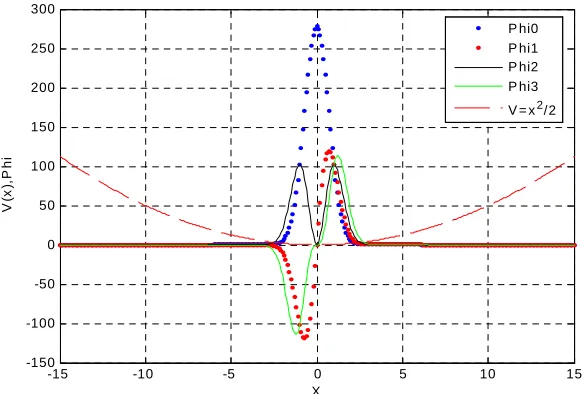
6.1. One Dimension Case (d = 1)
( )a We consider two class powers (shake power and light power) in (6.3), Setting shake power
e to the ground state solution and excite state of d- dimension BECS (Bose-Einstein condensate) with mix harmonic potential and crystal lattice potential.
The Gross-Pitaevskii equation:
21
2, 250, 2
V x x b b
taking initial wave
21 20
2 e
π
b
,
x
x
(6.4)
2
2 2
0 ,
i
, ,
2 r t h
t
h
V r NU r t r t
m
(6.1)
where d, 1, 2,3. 0,
rR d t m expresses mass of at
to calculate ground state g. For (6.4) we calculate first arouse state 1, space field for the time step for
10 x 10,
0.2. t
( )b Similar above way, taking
2
2
1
2 25sin π 4 , 500, 2,
V x x x b b
oms, h be planck constant, N be number of atoms in cohesion system, V r
be outer power,
2
0 4π
U h a m describe interaction between the at- oms cohesion (as 0, means repel; as0, shows
at appropriate im
and (6.3) for
21 20
2
: e
π
b
,
x
g x x
tract each other). Thus, by pass e (6.1) may be
measur- able process, then th written:
, 1 2
2
i
2 r t
V r r t r t
t
, , (6.2)
The parameter
and 10 x 10, and t 0.2.
On the other hand, by the MATLAB search the solu-tion of Equasolu-tion (6.3) in case (1) and (2) as follow with
0, , ,1 2 3
(See Figures 1 and 2).
tract corres
for positive, or negative, describe that repel or at ponding, out power V r
beby phys stem for us to s
a c
defined tudy things. By using
of the im ginary time method to alculate it in [22] that let it
ic sy 6.2. Two-Dimension Case (d = 2)
Consider shake power in [14,24]
substituting it into (6.2), we have
-15 -10 -5 0 5 10 15
-150 -100 -50 0 50 100 150 200 250 300
P hi0 P hi1 P hi2 P hi3
V = x2/2
V(
x
),
Ph
i
[image:8.595.153.444.519.716.2]X
, 0,0 ,0 ,, other.
x a y
V x y
b
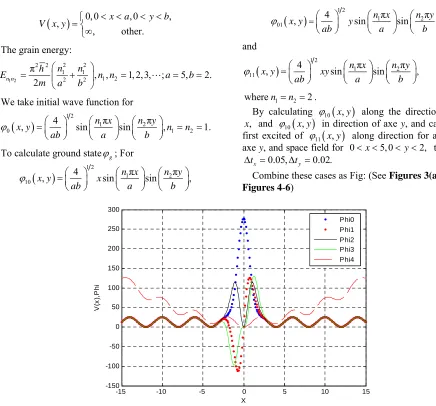
The grain energy:
1 2
2 2 2 2
1 1 1 2 2 2
π , , 1, 2,3, ; 5, 2.
2
n n
n n
h
E n n a
m a b
b
We take initial wave function for
1 2 1 20 1
π π
4
, sin n x sin n y ,
x y n n
ab a b
2 1.
To calculate ground stateg; For
1 2 1 210
π π
4
, sin n x sin n y
x y x
ab a b
1 2 1 201
π π
4
, sin n x sin n y
x y y
ab a b
,
and
1 2 1 211 ,
π π
4
, sin n x sin n y
x y xy
ab a b
1 2 wheren n 2.
10 x y,
By calculating along the direction of axe
,
x and 10
x y, cited ofin direction of axe y, and calculating first ex 11
x y, alld for
, and space fie
ong direction for axe x and
y 2, time step:
axe 0 x 5, 0 y
0.05, 0.02.
x y
t t
,
Figures 4-6) Combine these cases as Fig: (See Figures 3(a) and (b),
-15 -10 -5 0 5 10 15
-150 -100 -50 0 300
50 100 150 200 250
X
Phi0 Phi1 Phi2 Phi3 Phi4
V(
x
),
Ph
i
[image:9.595.66.502.81.487.2]2
Figure 2. Ground state phi0. First excited state phi1. V = x /2 + 25*(sin(pi*x/4))2; b = 500, bi = 2.
0 0.5 1 1.5 2 2.5 3 3.5 4 4.5 5 0
0.5 1 1.5 2 2.5 3 3.5 4 4.5 5
Phi0 Phi1 Phi2 Phi3
Ph
i
X
0 0.2 0.4 0.6 0.8 1 1.2 1.4 1.6 1.8 2 0
0.5 1 1.5 2 2.5 3 3.5 4 4.5 5
Y
P
hi
Phi0 Phi1 Phi2 Phi3
(b)
Figure 3. (a) Ground state phi0. First excited state phi1. a = 5, b = 2. (b) Ground state phi0. First excited state phi1. a = 5, b = 2.
0 1
2 3
4 5
0 0.5 1 1.5 2 0 0.5 1
X
Y
P
hi
[image:10.595.179.418.82.281.2]0
Figure 4. Ground state phi0 a = 5, b = 2.
0 1
2 3
4 5
0 0.5 1 1.5 2 -3 -2 -1 0 1 2 3
X
Y
P
hi
[image:10.595.174.419.323.714.2] [image:10.595.179.414.323.501.2]
0 1
2 3
4 5
0 0.5 1 1.5 2 -2 -1 0 1 2
X
Y
P
hi
[image:11.595.162.433.86.490.2] [image:11.595.167.430.87.277.2] [image:11.595.166.430.304.495.2]
Figure 6. First excited state phi2-y a = 5, b = 2.
0 1
2 3
4 5
0 0.5 1 1.5 2 -1.5 -1 -0.5 0 0.5 1 1.5
X
Y
P
hi
Figure 7. First excited state phi3-xy a = 5, b = 2.
We consider three-dimension case, Figure4 for ground state ϕ0
( )
x y, corresponding case, the ϕ10( )
x y, aswith express along direction of axe x (wave surface) in
Figure5, the ϕ01
( )
x y, as with express along directionof axe y (wave surface) in Figure 6, the ϕ11
( )
x y, asfor express along direction of axe x and axe y (wave sur- face) in Figure7.
7. Concluding Remarks
Recently, the higher-order Schrodinger differential equa- tions is also a very interesting topic, and that application of some physics and mechanics of for some more fields as nonlinear Schrodinger equations and some compute methods etc. In our future work, we may obtain some better results.
The application of some physics and mechanics of for some more fields with some combine equations (look [7,
13]).
8. Acknowledgements
This work is supported by the Nature Science Foundation (No.11ZB192) of Sichuan Education Bureau (No.11zd 1007 of Southwest University of Science and Technol- ogy).
REFERENCES
[1] B. L. Guo, “Initial Boundary Value Problem for One Class of System of Multi-Dimension Inhomogeneous GBBM Equation,” Chinese Annals of Mathematics, Vol. 8, No. 2, 1987, pp. 226-238.
[3] G. G. Cheng and J. Zhang, “Remark on Global Existence for the Superetitical Nonlinear Shrodinger Equation with a Harmonic Potential,” Journal of Mathematical Analysis and Applications, Vol. 320, No. 2, 2006, pp. 591-598.
[4] J. Zhang, “Blow-Up of Solutions to the Mixed Problems for Nonlinear Schrodinger Equations,” Journal of Si-chuan Normal University, Vol. 3, 1989, pp. 1-8.
[5] J. S. Zhao, Q. D. Guo, H. O. Yang and R. Z. Xu, “Blow-Up of Solutions for Initial Value Boundary Prob- lem of a Class of Generalized Non-Linear Schrodinger Equation,” Journal of Nature of Science of Heilongjiang University, Vol. 25, No. 2, 2008, pp. 170-172.
[6] N. H. Sweilam and R. F. AI-Bar, “Variational Iteration Method for Coupled Nonlinear Schrodinger Equations,”
Computers and Mathematics with Applications, Vol. 54, No. 7-8, 2007, pp. 993-999.
[7] J. Li and J. Zhan, “Blow-Up for the Stochastic Nonlinear Schrodinger Equation with a Harmonic Potential,” Ad- vances in Mathematics, Vol. 39, No. 4, 2010, pp. 491- 499.
[8] J. Zhang, “Sharp Conditions of Global Existence for Non- linear Schrodinger and Klein-Golden Equations,” Nonli- near Analysis, Vol. 48, No. 1, 2002, pp. 191-207.
[9] F. Genoud and C. A. Stuart, “Schrodinger Equations with a Spatially Decaying Non-Linear Existence and Stability of Standing Waves,” Discrete and Continuous Dynamical Systems, Vol. 21, No. 1, 2008, pp. 137-186.
[10] S. L. Xu, J. C. Liang and L. Yi, “Exact Solution to a Ge-neralized Nonlinear Schrodinger Equation,” Communica- tions in Theoretical Physics, Vol. 53, No. 1, 2010, pp. 159-165.
[11] H. Zhu, Y. Han and J. Zhang, “Blow-Up of Rough Solu- tions to the Fourth-Order Nonlinear Schrodinger Equa- tion,” Nonlinear Analysts,Vol. 74, No. 17, 2011, pp. 6186-
6201.
[12] H. Meng, B. Tian, T. Xu and H. Q. Zhang, “Backland Transformation and Conservation Laws for the Variable- Coefficient N-Coupled Schrodinger Equations with Sym- bolic Computation,” Acta Mathematica Sinica, Vol. 28, No. 5, 2012, pp. 969-974.
[13] G. R. Jia, J. C. Zhang, X. Z. Hang and Z. Z. Ren, “Cohe-rent Control of Population Transfer in Li Atoms via
Chirped Microwave Pulses,” Chinese Physics Letters, Vol. 26, No. 10, 2009, Article ID: 103201-1-4.
[14] N. H. Sweilam and R. F. Ai-Bar, “Variational Iterative Method for Coupled Nonlinear Schrodinger Equations,”
Computers and Mathematics with Applications, Vol. 54, No. 7-8, 2007, pp. 993-999.
[15] C. S. Zhu, “An Estimate of the Global Attractor for the Non-Linear Schrodinger Equation with Harmonic Poten- tial,” Journal of Southwest Normal university, Vol. 30, No. 5, 2005, pp. 788-791.
[16] B. L. Guo, T. Q. Han and X. N. Jie, “Existence of Global Smooth Solution to the Periodic Boundary of Fractional Non-Linear Schrodinger Equation,” Applied Mathematics and Computation, Vol. 204, No. 1, 2008, pp. 468-477.
[17] G. G. Lin and H. J. Gao, “Asymptotic Dynamical Differ- ence between the Nonlocal and Local Swift-Hohenberg Models,” Journal Mathematical Physics, Vol. 41, No. 4,
2000, pp. 2077-2089.
[18] L. Wang. J. B. Dang and G. G. Ling, “The Global At- tractor of the Fractional Nonlinear Schrodinger Equation and the Estimate of Its Dimension,” Journal of Yunnan University, Vol. 32, No. 2, 2010, pp. 130-135.
[19] V. G. Makhankov, “On Stationary Solutions of Schrod- inger Equation with a Self-Consistent Satisfying Boussi- nesq’s Equations,” Physics Letters A, Vol. 500, 1974, pp. 42-44.
[20] S. Zhang and F. Wang, “Inter Effects between There Cou- pled Bose-Einstein Condensates,” Physics Letters A, Vol. 279, 2001, pp. 231-238.
[21] A. Aftalion and Q. Do, “Vortices in A Rotating Bose- Einstein Condensate: Critical Angular Velocities and En- ergy Diagrams in the Thomas-Fermi regime,” Physics Letters A, Vol. 64, No. 6, 2001, Article ID: 063603.
[22] C. Tozzo, M. Kramer and F. Dalfovo, “Stability Diagram and Growth Rate of Parametric Resonances in Bose-Ein- stein Condensates in One Dimensional Optical Lattices,”
Physics Letters A, Vol. 72, No. 2, 2005, Article ID:
023613.
[23] J. Y. Zeng, “Quantum Mechanics,” Science Press, Beijing, 2004, pp. 33-144.
[24] R. Teman, “Infinite Dimensional Dynamical Systems in Mechanics and Physics,” Springer Verlag, New York,