Abstract—Exploration and investigation of clinical data reveals a number of issues, such as missing values, class imbalance and high dimensionality. This paper is motivated by these challenges especially imbalanced class, at the same time, maximising classification performance of data. A classifier often shows a strong bias toward the majority class, which is the negative case of patient in clinical datasets. Almost all classification methods used for have a strong bias towards the majority class, and are subject to error rates, e.g. false-negative rate implies that one of the performance indices, i.e. recall is often poor. Real live clinical data typically the proportion of positive cases is smaller than negative cases. Thus, a balance has to be restored using data sampling methods. This paper investigates methods of sampling, i.e. over-sampling and under-sampling to assess the performance of classification algorithms. Results show that each of the methods has a specific effect, it can be seen that under-sampling provides marginally better recall rates (sensitivity) by reducing the proportion of majority class and minimising the overall prediction error rate especially the minority class.
Index Terms— class balancing, sampling data, clinical data, recall
I. INTRODUCTION
EDICAL data commonly has an imbalanced class distribution, where one class is represented by a large number of samples while the others are represented by small numbers. Positive cases are special or rare cases that occur infrequently while negative cases are abundant. On such data learning classification methods generally perform poorly because the classifier often learns better the majority class. The reason for this is that learning classifiers attempt to reduce global quantities such as the error rate, and do not take the data distribution into consideration. As a result, samples from the dominant class are well-classified whereas samples from the minority class tend to be misclassified. There are two possible ways of improving the classification process, either the learning classification algorithms are modified or the data presented to them is modified.
The focus of this paper is on the modification of the data presented to the classifiers. Most machine learning algorithms (including learning classifiers) are trained based
Manuscript received March 25, 2014; revised April 10, 2014. N.Poolsawad would like to acknowledge the funding by the National Science and Technology Development Agency, Ministry of Science and Technology, Royal Thai Government for pursuing her research study.
N. Poolsawad is with the Computer Science, University of Hull, Cottingham Road Hull HU6 7RX UK ([email protected]).
C. Kambhampati is with the Computer Science, University of Hull, Cottingham Road Hull HU6 7RX UK (C.Kambhampati @hull.ac.uk).
J.G.F. Cleland is with the Cardiology, Hull York Medical School, University of Hull, Castle Hill Hospital Kingston upon Hull, HU16 5JQ, UK ([email protected]).
on the assumption that the ratios of each class are almost equal and thus the errors associated with each class have the same cost. Since the cost gets skewed in favour of the majority class, learning classifiers are often biased towards them. Thus, class balancing is the significant process to improve the data mining performance. In this paper, two strategies of sampling data, (1) over-sampling and (2) under-sampling, that will be solved this problem are outlined in section II. It should be noted that the size of samples for each class should be big enough to contain the significant information whether or be not too small to represent the data. A sampling strategy, which applies have to reveal a reliable, statistically representative sample of the full detail data. It is also advised to apply data sampling on imbalanced datasets for better accuracy performance.
II. CLASS BALANCING METHOD
Building a classification model with imbalanced dataset will cause the underrepresented class to be overlooked or even ignored. There are two techniques for balancing the classes, both of these change the ratios of the classes present and represent a re-sampling of available data. These are (a) oversampling and (b) under-sampling. These are discussed in the following sections.
A. Over-sampling strategy
Synthetic Minority Over-sampling Technique (SMOTE), developed by Chawla, Hall, & Kegelmeyer in 2002 [2], is an over-sampling technique whereby synthetic minority examples are generated. It combines informed over-sampling of the minority class with random under-over-sampling of the majority class. Using the over-sampling approach the minority class is over-sampled by creating artificial examples of k nearest class neighbours as seen in Fig. 1.
It has been shown that SMOTE yields better results for re-sampling and modifying the probabilistic estimate techniques [2]. This technique creates artificial samples to increase the size of minority class that is it has seen in Fig. 1. It balances the data by increasing the number of minority
Balancing Class for Performance of
Classification with a Clinical Dataset
N. Poolsawad, C. Kambhampati, and J.G.F. Cleland
M
[image:1.595.327.547.592.712.2]Synthetic instances
instances by over-sampling them. Thus SMOTE generates synthetic examples to the minority class; where the minority class is over-sampled by taking each minority class sample and introducing synthetic examples along the line segments joining any/all of the minority class nearest neighbours.
B. Under-sampling strategy
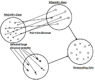
Another strategy of sampling data is under-sampling that reduces the set of data examples (in this paper means number of patients). The purpose of balancing data by using under-sampling is to achieve a high performance of classification and avoid the bias towards majority class examples [3]. One simple method for under-sampling data is to select a subset of majority class samples randomly [4, 5]. However, many researchers proposed different methods to select the samples from majority class for example, Near-miss methods [6], Cluster based method [5, 7, 8], and Distances between samples [5].
Here, distance-based random under-sampling is proposed and used to compare the performance of classification between over-sampling and under-sampling. The majority data is selected by using the pairwise distance; Euclidian distance is used in this paper but other distances can also be applied. This strategy also uses the similarity between the minority class and majority class to find the greatest distance between them as seen in Fig. 2. Then, majority class samples which high distance are selected to be balanced with minority class samples.
The relationship between training set size and improper classification performance for imbalanced data sets seems to be that on small imbalanced data sets the minority class is poorly represented by an excessively reduced number of examples that might not be sufficient for learning. For larger
data sets, the effect of these complicating factors seems to be reduced, as the minority class is better represented by a larger number of examples.
III. CLASSIFICATION BY SAMPLING OF CLINICAL DATASETS
A. Dataset
[image:2.595.326.518.149.217.2]Tests were carried out on a real live clinical data, and is a Heart Failure Dataset called “LIFELAB”. LIFELAB dataset [9-12] is dataset is a large repository of historical, and geographical covering generations of the same family and live clinical data. It’s a super set of SuperNova [13], TEN_HMS [14] and Heartcycle [15] datasets. In the paper a snap shot at a particular point of LIFELAB is used. It is composed of 60 features (variables), and 1,944 patients. Table I provides for further details of class distribution. The size of classes of target output, as shown in this table, is imbalanced.
B. Sampling techniques for clinical datasets
There is always in imbalance in real clinical datasets. The reason for this is that it is the norm that good (or alive) patients are more numerous than patients with ill-health (or dead). Thus, any framework for clinical datasets has to deal with this reality, there are two approaches that can be used, namely (a) over-sampling the minority class e.g. SMOTE, or (b) under sampling the majority class.
1) Over-sampling by SMOTE: As mentioned above, over sampling is essentially a process of generating new samples given an imbalanced dataset. One approach is to simply replicate the minority class n-number of times so that there is no major or minor class. This paper uses a more systematic approach to select some exemplars from the minority class, and then select extra samples by using nearest neighbours; often this is 3 depending on the ratio of the classes.
2) sampling by the samples distance: Under-sampling used in this paper selects samples from the majority class (‘Alive’ class) that are furthest from the minority class (‘Dead’ class) This is done using a Pairwise distance measure between the two classes (‘Dead’ and ‘Alive’ classes) of samples. For the purposes of this paper, the Euclidean distance measure has been used. However, if the data set was of a mixed type, other measures like the Mahalanobnis distance could be used.
C. Building the classifiers
The key to any algorithm within a data mining framework is its ability to provide correct information to the classification algorithms. In other words, the “goodness” of any methods for handling skews in classes, is judged on how well the resultant dataset is classified. The classifiers used to assess the performance are (a) Feed Forward Networks (MLPs) [16-18] (b) Radial Basis Function Networks (RBFN) [16] (c) Support Vector machines (SVMs) [19-21]
Algorithm for SMOTE
For each minority sample
Find its k-nearest minority neighbours Randomly select q of these neighbours
Randomly generate synthetic samples along the lines joining the minority sample and its q selected neighbours (q depends on the amount of oversampling desired)
Fig. 2: Under-sampling method
Algorithm for distance-based random under-sampling
For sample data in majority class
Apply Euclidian distance for the samples of majority and minority
Select the samples by finding the largest distance between minority ( ) and majority
Randomly select data sample from majority class that tend to be balanced with minority data
TABLEI
TARGET CLASSES DISTRIBUTION ON LIFELAB
No. of features 60
No. of samples 1944
Target output Mortality
Class Alive Dead
Frequency 1459 485
[image:2.595.85.253.346.487.2](d) Decision Trees (DT) [22] and (e) Random Forest (RF) [23, 24]. All of these methods are present in the software packages already mentioned.
D. Assessment of the data mining process
For clinical datasets, apart from the ability to predict the correct class, what is crucial is the number of false positives and false negatives and the amount of redundant information present within the dataset. Thus, in the evaluation in this paper, is carried out using two types of metrics (1) classification accuracy and (2) redundancy rate. Here, redundancy rate is used for assessing the subset of features from different feature selection methods [25].
Accuracy: Both Precision and Recall are used to assess the accuracy of the classifiers. These can be obtained from the data available in a confusion matrix. Both precision and recall are associated with false positives and false negatives. Thus for clinical datasets these two measure are significant [26, 27]. Two types of classification results are presented: 1) one with the 10-fold cross-validation and 2) a training set. The outcomes of classification which are used to form the confusion matrix are
True positive (TP):
A sample is predicted to be in class , and is actually in it. False positive (FP):
A sample is predicted to be in class , but is actually not in it. True negative (TN):
A sample is not predicted to be in class , and is actually not in it.
False negative (FN):
A sample is not predicted to be in class , but is actually in it.
In this paper precision and recall are measured the effectiveness of subset of features from different feature selection schemes [26-29]. Any single performance indicator suffers the risk of not being suitable; Fig. 3 and
Fig. 4 show that the relationship of performance indicators. Thus, we carefully used a confusion matrix to investigate and evaluate the performance of the classification. In medical diagnosis, the default assumption of equal misclassification costs underlying machine learning techniques is most likely violated. Precision is important that identified cases are true cases (high precision). A false negative prediction that is used for recall may have more serious consequences than a false positive prediction [30]. For example, consider prediction task, where we are predicting for patient who has a high probability of dead. Suppose that we are given a list of patients to classify as “relevant” or “non-relevant” for dead case, and then the cost of mistakenly assigning a relevant patient to the non-relevant patient class depends on whether there are any other relevant patents that we have correctly classified. Recall tends to be neglected or averaged away in machine learning and computational linguistics where the focus is on how confident we can be in the rule or classifier [26]. Consequently, in this paper both precision and recall are evaluated.
E. Results and discussions
The results presented here illustrate the data mining methods for handling the clinical data complexities. Data were pre-processed for analysis and then explored to discover data characteristics.
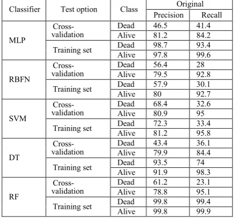
A set of initial benchmark results were obtained, using the ‘Original’ data (unpre-processing data). Table II shows the accuracy of the different classifiers when used on the ‘Original’ LIFELAB dataset, which consists of 60 variables, and contains missing values and imbalanced classes. From the results, it can be seen that the classifier based on the Random forest (RF) algorithm gives better accuracy than other classifiers, with more than 90% precision and recall for both classes. This is of course on the training set. RF is a versatile classification algorithm suited for the analysis of these large datasets and a suitable classification for clinical data [31-34] because RF classification models provide
Fig. 3: Relationship of performance indicators
TABLEII
THE CLASSIFICATION ACCURACY OF DIFFERENT CLASSIFICATIONS
USING ‘ORIGINAL’LIFELAB DATASET
Classifier Test option Class Original
Precision Recall
MLP
Cross-validation Dead Alive 46.5 81.2 41.4 84.2
Training set Dead Alive 98.7 97.8 93.4 99.6
RBFN
Cross-validation Dead Alive 56.4 79.5 28 92.8
Training set Dead Alive 57.9 80 30.1 92.7
SVM
Cross-validation Dead Alive 68.4 80.9 32.6 95
Training set Dead Alive 72.3 81.2 33.4 95.8
DT
Cross-validation Dead Alive 43.4 79.9 36.1 84.4
Training set Dead Alive 93.5 91.9 74 98.3
RF
Cross-validation
Dead 61.2 23.1
Alive 78.8 95.1
Training set Dead Alive 99.8 99.8 99.4 99.9
information on the importance of variables for the classification, leading to its superior performance on high-dimensional data [35, 36].
On the other hand, when checked with cross validation it can be seen that the performance is not as good. For example RF, precision and recall with the RF algorithm drops to 61.2% and 23.1%, for the ‘Dead’ class, and is at 78.8% and 95.1% for the ‘Alive’ class. A similar drop in precision and accuracy for all classes is exhibited by all the classifiers. For example SVM shows only a marginal improvement with precision of 68.4% and recall of 32.6% for the ‘Dead’ class, and 80.9% and 95% for the ‘Alive’ class. These differences are marginal at best. However, what is significant is that the accuracies associated with the ‘Alive’ class are higher than those for the ‘Dead’ class, and also the recall values on the ‘Dead’ class are significantly lower than precision values. This indicates that the ‘Alive’ class is better learnt than the dead class. This is a result of the existence of a far greater number of ‘Alive’ samples than ‘Dead’ samples. Hence, the data preparation is concerned in this research for any classification so missing values and imbalanced classes will be solved.
Typically, the proportion of positive and negative cases in a dataset is not equal (usually there are many more negative cases (‘Alive’ in our instance) than positive cases (‘Dead’ class)). This imbalance affects the learning process [37]. There are two approaches which can be applied here namely over- and under-sampling. These two sampling approaches change the number of positive or negative cases in the dataset to balance their proportions; Table III shows the result of these two sampling methods.
What is clear from the table is that both methods change the number of samples available. Over-sampling increases the ‘Dead’ class and thus increases the total number of sample, while under-sampling decreases the ‘Alive’ class sample and thus decreases the number of the total sample. It should be noted that under-sampling can result in the removal of important examples/exemplars from the dataset, whereas over-sampling can lead to overfitting [38]. According to previous studies [9-12, 39], the missing values issue is the one of vital problems e.g. class imbalanced, high dimensions, in this dataset, then SVMI [40] is used to be the representative for missing values imputation. SVMI would also be useful to attempt to find heuristics to characterize the data that would act as a guide for choosing the most appropriate imputation method [40, 41] and also it is recommended for the processing of clinical data [39, 42]. Given the performance of SVM based imputation, it is only natural to use this scheme for all future results and analysis. This method reflects the hidden information in the whole data in contrast to other methods, such as by assuming that the missing points are the same as their nearest neighbours, where local information is taken into account, resulting in bigger errors. [40]. It is also evident that the imputation
scheme based on SVMs provides greater improvements in the performance of classification algorithms.
From the results in Table IV it can be seen that that the recall values for the ‘Dead’ class are relatively low compared to the ‘Alive’ class. This could be the result of the presence of large amount of missing values and the imbalance of classes. Missing values could be compounding the class imbalance more for the dead class than the ‘Alive’ class. From both the tables (Tables II and IV) it can be seen
TABLEIII
THE LIFELAB WITH DIFFERENT RESAMPLING METHODS
Resampling No. of
patient
Class No. of patient
Imbalanced 1944 Alive Dead 1459 485
Over-sampling 2429 Alive Dead 1459 970
Under-sampling 1009 Alive Dead 524 485
TABLEIV
THE CLASSIFICATION ACCURACY ON IMBALANCED AND BALANCED DATA
Data Classification option Test Class Precision Recall
Imb al an ce d MLP Cross-validation
Dead 53.2 46.6
Alive 82.9 86.4
Training set
Dead 96.1 81
Alive 94 98.9
RBFN
Cross-validation
Dead 60.9 32.4
Alive 80.5 93.1
Training set
Dead 63.4 32.2
Alive 80.6 93.8
SVM
Cross-validation
Dead 68.9 36.1
Alive 81.7 94.6
Training set
Dead 74.2 39.8
Alive 82.7 95.4
DT
Cross-validation
Dead 55.9 53
Alive 84.6 86.1
Training set
Dead 97.6 92.8
Alive 97.6 99.2
RF
Cross-validation
Dead 69.3 56.3
Alive 86.3 91.7
Training set
Dead 99.6 100
Alive 100 99.9
O ve r-sam pl in g MLP Cross-validation
Dead 70.2 70
Alive 80.1 80.3
Training set
Dead 81 96.2
Alive 97.1 85
RBFN
Cross-validation
Dead 67.2 66.8
Alive 78 78.3
Training set
Dead 68.8 67.8
Alive 78.8 79.6
SVM
Cross-validation
Dead 74.8 66.3
Alive 79.2 85.1
Training set
Dead 76.6 67.5
Alive 80 86.3
DT
Cross-validation
Dead 70 69.9
Alive 80 80.1
Training set
Dead 97.8 98.2
Alive 98.8 98.6
RF
Cross-validation
Dead 77.6 79.8
Alive 86.3 84.6
Training set
Dead 100 99.9
Alive 99.9 100
U nd er -samp lin g MLP Cross-validation
Dead 73 70.8
Alive 69.5 71.8
Training set
Dead 98.3 98.1
Alive 97.9 98.1
RBFN
Cross-validation
Dead 70.9 71
Alive 68.6 68.5
Training set
Dead 74.8 71.8
Alive 70.8 73.8
SVM
Cross-validation
Dead 73.9 74.6
Alive 72.3 71.5
Training set
Dead 76.8 76.5
Alive 74.7 75.1
DT
Cross-validation
Dead 74.4 75.4
Alive 73 72
Training set
Dead 97.2 98.5
Alive 98.3 96.9
RF
Cross-validation
Dead 75.3 82.6
Alive 79 70.7
Training set
Dead 99.6 100
that there is an improvement in accuracy when missing values are imputed. What can be seen within the details is that precision improves significantly but recall does not improve at the same level. It should be noted that “precision” is associated with false positive while “recall” is false negative classification, and thus for clinical application recall becomes important. Given the lack of a sufficient number of samples in this class, imputation can only improve it by small amounts.
Table IV compares three different sets of results. The first set is the classification performance using the imbalanced dataset and the next two are based on the balancing approaches taken. It can be seen that balancing the classes greatly improves the performance of the algorithms. The key indicator of recall shows a significant improvement with all classification algorithms. Thus balancing of classes does lead to better performance in all indicators but shows significant improvement in the key indicators. For example, with the RF classification, precision on ‘Dead’ Class rises from 69.3% to 77.6% using oversampling, and 75.3% with under-sampling, while recall changes from 56.3% to 79.8% and 82.6%. However, this table also illustrates the issue of reducing dimensions before balancing is carried out. Although it can be argued that the variable set is not an optimal one; it is nevertheless one used by expert clinicians. What can be concluded is that both the sampling methods improve classification [43], since classifiers are often biased towards the majority class [44]. A key focus should be the effect of the individual strategy on rates of recall, and it can be seen that under-sampling provides marginally better recall rates.
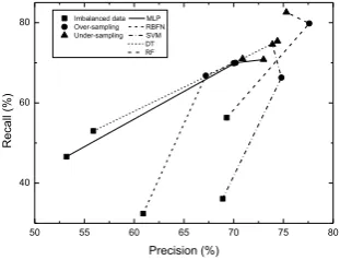
Fig. 5 represents the results of cross-validation of different classifiers from Table IV that comparing the precision and recall of different classifiers on imbalanced and balanced (over-sampling and under-sampling) data. The results illustrate that the balanced data after applying sampling methods, greatly improves the performance; especially recall (steep slopes) values. As a result, the sampling strategies were validated by comparison of different classifiers reveal that an under-sampling may be more suitable for clinical datasets, as it reduces the proportion of negative cases and keeps the positive cases, at the same time the error rates of minority class (positive case) are minimised.
The graphs in Fig. 6 (a-b) and Fig. 7 (a-b) illustrate the above analysis further. These graphs show the changes to precision and recall, under three different conditions, namely: original data set, dataset with imputation and dataset with different sampling strategies. It can be seen that improvements are made progressively at each stage. It can be seen that there are sharp increases after sampling the data
post imputation. Fig. 6 (a) and Fig. 7 (a) show that precision from both sampling have a slightly different improvement. Fig. 6 (b) and Fig. 7 (b) show that under-sampling provides improved marginally better recall rates than over-sampling.
IV. CONCLUSIONS
A sampling strategy, which is applied, has to be such that reliable results are obtained, and is also, statistically representative of the full detail data. This rules must be kept in mind for most datasets, more so for clinical datasets, where imbalance is factor and throwing away of valuable information is always possible when resampling the data. Imbalanced class is an issue that does occur naturally in clinical datasets. Resampling of data sampling is one way to deal with this problem and is essentially a process which enables the balancing of the proportions of majority and minority class in a dataset, such that they both have similar sizes in terms of number of samples in each class. A key reason for this resampling is that most data mining and classification algorithms often show a strong bias towards the majority class, and for purposes of clinical applications a goal is to minimise the overall prediction error rate especially the minority class (positive case). The results presented in this paper showed that balancing the dataset, greatly improves the performance; especially recall (sensitivity) values. Indeed, the sampling strategies and the analysis of the previous section were further validated by comparison of different classifiers. A conclusion is that as a strategy under-sampling may be more suitable for clinical datasets, as it reduces the proportion of negative cases and keeps the positive cases, at the same time the error rates of minority class (positive case) are minimized. It should be noted that the size of samples for each class should be big enough to contain the significant information whether or be not too small to represent the data.
REFERENCES
[1] T. Borovicka, M. Jirina, Jr., and P. Kordik, Selecting Representative
Data Sets, 2012.
50 55 60 65 70 75 80
40 60
80 Imbalanced data MLP Over-sampling RBFN Under-sampling SVM DT RF
Recall
(%)
[image:5.595.317.549.190.280.2]Precision (%)
Fig. 5: The classification accuracy on imbalanced and balanced data
Original Imputed Balanced 40
45 50 55 60 65 70 75
(a) Precision
Precision
(%)
Dataset
MLP RBFN SVM DT RF
Original Imputed Balanced 20
30 40 50 60 70 80 90
Recall (
%)
Dataset
MLP RBFN SVM DT RF
(b) Recall
Fig. 7 (a-b): The classification accuracy on data mining process for under-sampling
Original Imputed Balanced 40
45 50 55 60 65 70 75 80
(a) Precision
MLP RBFN SVM DT RF
Precision
(%)
Dataset
Original Imputed Balanced 20
30 40 50 60 70 80
(b) Recall
MLP RBFN SVM DT RF
Recall (
%)
Dataset
[image:5.595.87.243.416.535.2][2] N. V. Chawla, K. W. Bowyer, L. O. Hall, and W. P. Kegelmeyer,
"SMOTE: synthetic minority over-sampling technique," J. Artif. Int.
Res., vol. 16, pp. 321-357, 2002.
[3] S. Garcia and F. Herrera, "Evolutionary undersampling for
classification with imbalanced datasets: proposals and taxonomy," Evol
Comput, vol. 17, pp. 275-306, 2009.
[4] Z. Yan-ping, Z. Li-Na, and W. Yong-Cheng, "Cluster-based majority under-sampling approaches for class imbalance learning," in
Information and Financial Engineering (ICIFE), 2010 2nd IEEE International Conference on, 2010, pp. 400-404.
[5] S.-J. Yen and Y.-S. Lee, "Cluster-Based Sampling Approaches to
Imbalanced Data Distributions," in Data Warehousing and Knowledge
Discovery. vol. 4081, A. Tjoa and J. Trujillo, Eds., ed: Springer Berlin Heidelberg, 2006, pp. 427-436.
[6] J. Zhang and I. Mani, "KNN Approach to Unbalanced Data Distributions: A Case Study Involving Information Extraction," in
ICML'2003 Workshop on Learning from Imbalanced Datasets, 2003. [7] H. Altınçay and C. Ergün, "Clustering Based Under-Sampling for
Improving Speaker Verification Decisions Using AdaBoost," in
Structural, Syntactic, and Statistical Pattern Recognition. vol. 3138, A. Fred, T. Caelli, R. W. Duin, A. Campilho, and D. de Ridder, Eds., ed: Springer Berlin Heidelberg, 2004, pp. 698-706.
[8] M. M. Rahman and D. N. Davis, "Cluster Based Under-Sampling for
Unbalanced Cardiovascular Data," in World Congress on Engineering
2013, London, UK, 2013.
[9] N. Poolsawad, L. Moore, C. Kambhampati, and J. G. F. Cleland, "Performance Metrics for Classification in Clinical Dataset," presented at the the 19th International Conference on Neural Information Processing (ICONIP2012), Doha, Qatar, 2012.
[10] N. Poolsawad, L. Moore, C. Kambhampati, and J. G. F. Cleland, "Handling Missing Values in Data Mining - A Case Study of Heart
Failure Dataset," in The 2012 8th International Conference on Natural
Computation (ICNC'12) and the 2012 9th International Conference on Fuzzy Systems and Knowledge Discovery (FSKD'12), Chongqing, China, 2012, pp. 2946-2950.
[11] N. Poolsawad, C. Kambhampati, and J. G. F. Cleland, "Feature Selection Approaches with Missing Values Handling for Data Mining -
A Case Study of Heart Failure," in International Conference on Data
Mining (ICDM 2011), Phuket, Thailand, 2011, pp. 828-836.
[12] N. Poolsawad and C. Kambhampati, "Issues in the mining of heart
failure datasets," International Journal of Automation and Computing,
vol. 11, pp. 162-179, 2014.
[13] P. A. Poole-Wilson, K. Swedberg, J. G. Cleland, A. Di Lenarda, P. Hanrath, M. Komajda, J. Lubsen, B. Lutiger, M. Metra, W. J. Remme, C. Torp-Pedersen, A. Scherhag, and A. Skene, "Comparison of carvedilol and metoprolol on clinical outcomes in patients with chronic heart failure in the Carvedilol Or Metoprolol European Trial
(COMET): randomised controlled trial," Lancet, vol. 362, pp. 7-13,
2003.
[14] J. G. Cleland, A. A. Louis, A. S. Rigby, U. Janssens, and A. H. Balk, "Noninvasive home telemonitoring for patients with heart failure at high risk of recurrent admission and death: the Trans-European
Network-Home-Care Management System (TEN-HMS) study," J Am
Coll Cardiol, vol. 45, pp. 1654-64, 2005.
[15] H. Reiter and N. Maglaveras, "HeartCycle: compliance and
effectiveness in HF and CAD closed-loop management," Conf Proc
IEEE Eng Med Biol Soc, p. 5333151, 2009.
[16] K. Suzuki, Artificial Neural Networks - Methodological Advances and
Biomedical Applications. Rijeka, Croatia: InTech, 2011.
[17] M. W. Gardner and S. R. Dorling, "Artificial neural networks (the multilayer perceptron)—a review of applications in the atmospheric
sciences," Atmospheric Environment, vol. 32, pp. 2627-2636, 1998.
[18] L. Autio, M. Juhola, and J. Laurikkala, "On the neural network classification of medical data and an endeavour to balance non-uniform
data sets with artificial data extension," Computers in Biology and
Medicine, vol. 37, pp. 388-397, 2007.
[19] C. Cortes and V. Vapnik, "Support-Vector Networks," Machine
Learning, vol. 20, pp. 273-297, 1995/09/01 1995.
[20] J. C. Platt, "Fast training of support vector machines using sequential
minimal optimization," in Advances in kernel methods, ed MA, USA:
MIT Press, 1999, pp. 185-208.
[21] T. Hastie and R. Tibshirani, "Classification by pairwise coupling," presented at the Proceedings of the 1997 conference on Advances in neural information processing systems 10, Denver, Colorado, USA, 1998.
[22] J. R. Quinlan, "Improved use of continuous attributes in C4.5," J. Artif.
Int. Res., vol. 4, pp. 77-90, 1996.
[23] L. Breiman, "Bagging Predictors," Mach Learn, vol. 24, pp. 123 - 140,
1996.
[24] L. Breiman, "Random forests," Mach Learn, vol. 45, pp. 5 - 32, 2001.
[25] Z. Zhao and L. Wang, "Efficient Spectral Feature Selection with
Minimum Redundancy," in Twenty-Fourth AAAI Conference on
Artificial Intelligence, AAAI 2010, Atlanta, Georgia, USA, 2010. [26] D. Powers, "Evaluation: From Precision, Recall and F-Factor to ROC,
Informedness, Markedness & Correlation," School of Informatics and Engineering, Flinders University of South Australia Adelaide, AustraliaDecember 2007.
[27] G. Forman, "An Extensive Empirical Study of Feature Selection
Metrics for Text Classification," Journal of Machine Learning
Research, vol. 3, pp. 1289-1305, 2003.
[28] P. Cheong Hee, P. Haesun, and P. Pardalos, "A comparative study of
linear and nonlinear feature extraction methods," in Data Mining,
2004. ICDM '04. Fourth IEEE International Conference on, 2004, pp. 495-498.
[29] P. Turney, "Types of cost in inductive concept learning," in
Seventeenth International Conference on Machine Learning, ed, 2000. [30] F. Yang, H.-z. Wang, H. Mi, C.-d. Lin, and W.-w. Cai, "Using random
forest for reliable classification and cost-sensitive learning for medical
diagnosis," BMC Bioinformatics, vol. 10, p. S22, 2009.
[31] T. Chen, Y. Cao, Y. Zhang, J. Liu, Y. Bao, C. Wang, W. Jia, and A. Zhao, "Random Forest in Clinical Metabolomics for Phenotypic
Discrimination and Biomarker Selection," Evidence-Based
Complementary and Alternative Medicine, vol. 2013, p. 11, 2013. [32] C. Strobl, A. Boulesteix, T. Kneib, T. Augustin, and A. Zeileis,
"Conditional variable importance for random forests," BMC
Bioinformatics, vol. 9, p. 307, 2008.
[33] U. Diaz and A. Alvarez, "Gene Selection and Classification of
Microarray Data Using Random Forest," BMC Bioinformatics, vol. 7,
p. 3, 2006.
[34] H. Pang, A. Lin, M. Holford, B. E. Enerson, B. Lu, M. P. Lawton, E. Floyd, and H. Zhao, "Pathway analysis using random forests
classification and regression," Bioinformatics, vol. 22, pp. 2028-2036,
2006.
[35] L. Breiman, "Consistency for a Simple Model of Random Forests,," Statistics Department, University of California Berkeley2004. [36] W. G. Touw, J. R. Bayjanov, L. Overmars, L. Backus, J. Boekhorst, M.
Wels, and S. A. van Hijum, "Data mining in the Life Sciences with
Random Forest: a walk in the park or lost in the jungle?," Brief
Bioinform, vol. 14, pp. 315-26, 2013.
[37] H. He and E. A. Garcia, "Learning from Imbalanced Data," IEEE
Trans. on Knowl. and Data Eng., vol. 21, pp. 1263-1284, 2009. [38] D. Mease, A. J. Wyner, and A. Buja, "Boosted Classification Trees and
Class Probability/Quantile Estimation," Journal of Machine Learning
Research, vol. 8, pp. 409-439, 2007.
[39] Y. Zhang, C. Kambhampati, D. N. Davis, K. Goode, and J. G. F. Cleland, "A Comparative Study of Missing Value Imputation with
Multiclass Classification for Clinical Heart Failure Data," in The 2012
8th International Conference on Natural Computation (ICNC'12) and the 2012 9th International Conference on Fuzzy Systems and Knowledge Discovery (FSKD'12), Chongqing, China, 2012, pp. 2946-2950.
[40] F. Honghai, C. Guoshun, Y. Cheng, Y. Bingru, and C. Yumei, "A SVM regression based approach to filling in missing values," presented at the Proceedings of the 9th international conference on Knowledge-Based Intelligent Information and Engineering Systems - Volume Part III, Melbourne, Australia, 2005.
[41] H. Mallinson and A. Gammerman, "Evaluation of Support Vector Machines for Imputation," Department of Computer Science, Royal Holloway, University of London2005.
[42] H. Wang and S. Wang, "Mining incomplete survey data through
classification," Knowledge and Information Systems, vol. 24, pp.
221-233, 2010/08/01 2010.
[43] R. Hunt, M. Johnston, W. Browne, and M. Zhang, "Sampling Methods in Genetic Programming for Classification with Unbalanced Data," in
AI 2010: Advances in Artificial Intelligence. vol. 6464, J. Li, Ed., ed: Springer Berlin Heidelberg, 2011, pp. 273-282.
[44] Z. Afzal, M. Schuemie, J. van Blijderveen, E. Sen, M. Sturkenboom, and J. Kors, "Improving sensitivity of machine learning methods for automated case identification from free-text electronic medical
records," BMC Medical Informatics and Decision Making, vol. 13, pp.
![Fig. 1: SMOTE - synthetic instances [1]](https://thumb-us.123doks.com/thumbv2/123dok_us/457816.543805/1.595.327.547.592.712/fig-smote-synthetic-instances.webp)