On the effects of nonequilibrium on the subgrid scale stresses

On the effects of nonequilibrium on the subgrid-scale stresses

Ugo Piomelli

Department of Mechanical Engineering, University of Maryland, College Park, Maryland 20742

Gary N. Coleman and John Kim

Department of Mechanical and Aerospace Engineering, University of California, Los Angeles, California 90095-1597

~Received 17 December 1996; accepted 17 April 1997!

An a priori study of the subgrid-scale ~SGS! stresses and dissipation in two nonequilibrium, wall-bounded flows is carried out. The velocity fields were computed by direct simulations of two-and three-dimensional boundary layers obtained, respectively, by a sudden change in the Reynolds number and by an impulsive motion in the spanwise direction of the lower wall of a plane channel in fully developed turbulent flow conditions. Several realizations of the transient period of the flow were examined. The SGS stresses react to the imposition of the secondary shear more rapidly than the large-scale ones, and return to equilibrium before the resolved stresses do. In general, the subgrid scales are less sensitive than the large ones to the near-wall and nonequilibrium effects. Scale-similar and dynamic models appear well-suited to reproduce the correlation between resolved Reynolds stress production and events with significant production of SGS energy. © 1997 American Institute of Physics. @S1070-6631~97!01208-7#

I. INTRODUCTION

Large-eddy simulations ~LES! of the Navier–Stokes equations are based on the assumption that the small, subgrid scales of motion are more universal than the large, energy-carrying ones, less affected by the boundary conditions, and, therefore, easier to model. Since in LES only the largest structures are computed, coarser grids can be used than in direct simulations, and higher Reynolds number flows can be studied at a fraction of the expense. Moreover, the modeling of the small scales in principle is simpler than the modeling of all the scales of motions required by Reynolds-averaged

~RANS! calculations, and, therefore, better accuracy can be achieved, especially in three-dimensional flows for which most turbulence models ~especially two-equation models! are known to be inadequate.

Since the small scales tend to be more homogeneous and isotropic than the large ones, simple models should be able to describe their physics fairly accurately. Furthermore, since the subgrid-scale ~SGS!stresses are a small fraction of the total stresses, modeling errors should not affect the overall accuracy of the results as much as in the Reynolds-averaged turbulence modeling approach. For these reasons, most sub-grid scale models in use presently are eddy-viscosity models that relate the subgrid-scale stresses, ti j, to the large-scale

strain-rate tensor S¯i j. The eddy viscosity is given by the

product of a length scale,

l

the most active unresolved scales are those closest to the cutoff, the natural length scale in LES modeling is the filter width, which is representative of the size of the smallest resolved structure in the flow, and is typically proportional to the grid size. The velocity scale is usually taken to be the square root of the trace of the SGS stress tensor, q_sgs2 5tkk. To determine qsgs

2

in most cases the equilibrium assumption is exploited to obtain an algebraic model for the eddy viscosity.1

The Smagorinsky model can be derived2 based on the

observation that the small scales of motion have shorter time scales than the large, energy-carrying eddies; for this reason, it can be assumed that they adjust more rapidly than the large scales to perturbations, and recover equilibrium nearly in-stantaneously. Under this assumption, the transport equation for q_sgs2 reduces to2ti j¯Si j5«v, where2ti j¯Si j is the

pro-duction, and«_v the viscous dissipation, of SGS energy. The negative of the production term, «sgs5ti j¯Si j, is often

re-ferred to as the ‘‘SGS dissipation,’’ since it also represents the dissipation of resolved energy by the SGS stresses. This balance, together with the definition of the eddy viscosity, can be used to obtain the velocity scale.

The equilibrium assumption implies inertial range dy-namics: energy is generated at the large-scale level and trans-mitted to smaller and smaller scales, where the viscous dis-sipation takes place. Very little testing of the applicability of this assumption to the small scales of turbulence is available. It is well known that in most flows of interest the large scales are not in equilibrium: Smith and Yakhot3studied the short-time behavior of the eddy viscosity in the Reynolds-averaged framework, and found thatK2« models do not predict the correct response of the eddy viscosity if homogeneous iso-tropic turbulence is suddenly subjected to a perturbation

complex flows, in which extra strains, backscatter, intermit-tency, and other phenomena play a role, it is not known whether the small scales would still be represented ad-equately by equilibrium-based subgrid-scale models.

The purpose of this paper is to study the physical behav-ior of the subgrid scales of motion in situations of strong perturbation from equilibrium by a priori testing. Two cases will be studied: The first is a fully developed plane channel flow in which the viscosity is suddenly decreased to acceler-ate the flow, which reaches equilibrium at a higher Reynolds number; the second, a three-dimensional, shear-driven boundary layer,5 obtained by moving the lower wall of a fully developed plane channel flow in the spanwise direction. Both flows are initially equilibrium flows that approach an-other equilibrium state, and thus allow comparison of the response of both large and subgrid scales to the perturbation, and their return to equilibrium.

Furthermore, the performance of several models will be compared. The models chosen are the Smagorinsky model,1 the dynamic eddy-viscosity model,6,7 and two scale-similar models.8,9Both the Smagorinsky and the dynamic model are eddy-viscosity models; the model coefficient in the former is set a priori, while in the latter it is adjusted according to the energy content of the simulation. Thus the dynamic model should be able to adjust more rapidly than the Smagorinsky model to the perturbations. Scale-similar models use the smallest resolved scales to parametrize the unresolved ones. They are based on the hypothesis that the most important interactions between resolved and unresolved scales occur between the eddies closest to the cutoff wave number. This dependence on the model on the smallest resolved scales will also be shown to have beneficial effects for the prediction of the response of the SGS stresses to perturbations.

In the next section the governing equations and the mathematical approach will be presented. The results of the a priori test will be presented is Sec. III. Some conclusions will be drawn in the last section.

II. PROBLEM FORMULATION

A. Governing equations

In LES dependent flow variables are divided into a grid-scale~GS! part and a subgrid-scale~SGS!part by the filter-ing operation

f ¯_~x!5

E

D

f~x

8

8

8

where D is the computational domain, and G is the filter function. The application of this operation to the continuity and Navier–Stokes equations yields the equations that gov-ern the evolution of the large, energy-carrying scales of mo-tion:

]¯ui

]t 1

]

]x_j~¯ui¯uj!52 1

r ]¯p

]x_i2

]ti j ]x_j1n

]2_¯u i

]x_j]x_j, ~2!

]¯ui ]xi5

0, ~3!

where x ~or x1) is the streamwise direction, y ~or x2) the

wall–normal direction, and z ~or x3) the spanwise direction;

u, v, and w ~or u1, u2, and u3) are the velocity components

in the coordinate directions. The effect of the small scales appears in the SGS stress term, ti j5u¯iuj2¯ui¯uj, which

must be modeled.

B. Subgrid-scale stress models

In the past, two main types of models have been used to parametrize the SGS stresses: eddy viscosity and scale-similar models. Eddy-viscosity models represent the aniso-tropic part of the SGS stress tensor as

ti j2 di j

3 tkk522nT¯Si j, ~4!

where n_T is the eddy viscosity and S¯_{i j} is the large-scale strain rate tensor

S ¯

i j5

1

2

S

]¯ui ]xj

1]¯uj ]xi

D

. ~5!

The assumption that2ti j¯Si j5«v, where

«v5

S

]xj ]u_i

]xj2 ]¯u_i

]xj ]¯u_i

]xj

D

, ~6!

allows the eddy viscosity to be written as1

nT5~CSD!2u¯Su, ~7!

where u¯Su5(2 S¯i j¯Si j)1/2, D is the ~grid-scale! filter width,

and the Smagorinsky constant, CS, can be determined by

integrating the vorticity spectrum function over all the unre-solved wave numbers.2In practice, the value of the constant is substantially reduced in the presence of shear, and van Driest10damping is used to account for near-wall effects; the eddy viscosity thus becomes

nT5@CSD~12e2y

1_/25

!#2_{u¯Su, ~8!}

where y15y_wu_t/n, y_w is the distance from the wall, and C_s.0.06520.1.

Recently, dynamic models have been introduced that ad-just the coefficient locally and instantaneously from the en-ergy content of the smallest resolved scales.6These are gen-erally Smagorinsky-like models in which the coefficient C is determined based on the energy content of the smallest re-solved scales of motion. In this work, the plane-averaged formulation,7 which has been applied successfully to the simulation of transitional and turbulent plane channel flows6,11will be used, in which the SGS stresses are given by

~4!, withnT5CD2u¯Su, and

C521 2

^

&

^

&

, ~9!

where

^

&

the wall, Li j5¯dui¯uj2¯uˆi¯uˆj are the resolved turbulent

Scale similar models also use the energy content of the smallest resolved scales of motion to predict the behavior of the SGS stresses. In this work, two such models will be tested, the one originally developed by Bardina et al.:8

ti j5¯ui¯uj2¯¯ui¯¯uj ~10!

and the one recently proposed by Liu et al.:9

ti j5CLLi j; ~11!

Liu et al.9 recommended a value C_L50.45. The coefficient can also be adjusted dynamically.

C.A priori tests

In a priori tests the resolved velocity fields obtained from direct simulations of the Navier–Stokes equations are filtered explicitly according to ~1! to yield the exact SGS quantities of interest. Two filter functions are considered in this study: the sharp cutoff filter in Fourier space and the box

~or tophat! filter in physical space. The sharp cutoff filter is best defined in Fourier space as:

g~k!5

E

D

G~x

8

85

H

1, if k<p/D,

0, otherwise, ~12!

while the box~or top hat!filter is

G~x!5

H

1/D, if uxu<D/2,

0, otherwise. ~13!

Three DNS databases were used in this work: the first is the DNS of a two-dimensional plane channel flow at Re_t5180 ~based on friction velocity u_t and channel half-width d), computed using a pseudo-spectral code with 1283973128 grid points and a computational domain of 4pd32d34pd/3. The results of this calculation were shown by Piomelli et al.12to be in good agreement with the direct numerical simulations ~DNS!of Kim et al.13 The ac-celerating channel case was computed using the same pseudo-spectral code; the flow was started from a steady-state field at Re_t5150 ~based on the initial friction velocity u_t,o and viscosityno); the Reynolds number was then

sud-denly increased, and a new equilibrium state was reached at Re_t5225 at tu_t,o/d.1.2.

The shear-driven three-dimensional boundary layer ve-locity fields were obtained from the calculations by Coleman et al.5using the spectral code of Kim et al.13 The computa-tional domain was 4pd32d38pd/3 in the streamwise (x₁ or x), wall-normal (x₂ or y ), and spanwise (x₃ or z) direc-tions, respectively, and 25631293256 grid points were used. An impulsive spanwise motion, with magnitude equal to 47% of the initial mean centerline velocity, was applied to the lower wall of a fully developed plane channel flow; the initial condition was obtained from the calculation at Rey-nolds number Re_t5180. The flow was allowed to develop until a collateral state~one in which the new direction of the mean velocity is the same at each y ) was reached. Notice that, since periodic boundary conditions were used, the boundary layer due to the spanwise motion of the wall grows in time rather than in space.

The exact GS and SGS fields were obtained by filtering the DNS data over the streamwise and spanwise homoge-neous directions using different filter types and sizes. A typi-cal test performed using the Fourier cutoff filter employs a filter width Di54Dxi ~for i51 and 3!; for the box filter

widths Di52Dxi andDi54Dxi were used. With these

val-ues, the ratio of SGS to total fluctuating energy was 15%– 25%, a range representative of actual LES calculations. No significant difference was observed between the results for the two filters.

All the data shown in the following were averaged over several realizations of the flow fields in question, as well as over planes parallel to the wall. Since the expense required to generate ensembles of data in this type of unsteady flows is significant, the sample size in some cases is insufficient to obtain fully converged results. However, the purpose of the a priori test is only to supply physical insight into the phenom-ena that affect the subgrid scales and identify the trends; for this purpose, the sample size is adequate.

Two normalizations will be used: one in which all quan-tities are made dimensionless using the initial friction veloc-ity u_t,o and molecular viscosity n_o. In the other the time-dependent values of the friction velocity u_t and viscosityn are used. Quantities made dimensionless by the latter nor-malizations will be denoted by a prime.

III. RESULTS AND DISCUSSION

A. Plane channel flow

In Fig. 1 the terms in the budget of the SGS kinetic energy Ksgs5tkk/2 are shown for the two-dimensional

kinetic energy, at this Reynolds number, production and dis-sipation are not in balance near the wall, where the various diffusion terms are significant;14 in the outer region the tur-bulent transport term is not negligible. Only at much higher Reynolds number does behavior like that observed here for the SGS energy become apparent. This point further supports the equilibrium assumption for the small scales.

When homogeneous turbulence is suddenly subjected to mean shear, its short-time response is characterized by a lag between the imposition of the strain and the increase in tur-bulent kinetic energy due to the increased production. Smith and Yakhot3accounted for the lag, within the framework of

K2« models, by introducing an exponential correction to the eddy viscosity, which includes a time constant, the eddy turnover time t;K/«. In the context of LES, in which the SGS model only represents the scales smaller than the filter width, a relevant eddy turnover time must be defined in terms of SGS quantities only, and could depend on the filter width. In Fig. 2 such an eddy turnover time, defined in terms of Ksgs and«v is shown as a function of distance from the

wall for the two-dimensional channel; the Fourier cutoff fil-ter was used. The plane-averaged values (Di→`) are equivalent to long-time averages and thus represent the eddy turnover time relevant to K2« models. Both SGS energy and viscous dissipation decrease as the filter width is de-creased; the SGS turnover time is, however, fairly indepen-dent of the filter width, and, except very near the wall, is equal to about 50%–60% of the Reynolds-averaged turnover time. While the subgrid scales can be expected to react more rapidly than the largest scales of motion, their response to a perturbation is not instantaneous. Accounting for this adjust-ment time could improve significantly the accuracy of SGS stress models.

B. Accelerating channel flow

In the accelerating channel flow the perturbation that dis-rupts the equilibrium state consists of a sudden increase of

the Reynolds number. Consequently, one would expect the high-wave-number region of the velocity spectra to fill up, and the small scales should be affected more than the large ones by the perturbation.

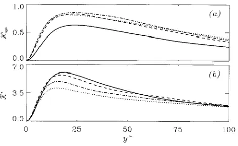
In Fig. 3 large-scale and SGS kinetic energy profiles are shown at various times during the transient. While the maxi-mum total kinetic energy,K¯1Ksgs increases only by 25%,

the subgrid-scale energy increases by more than a factor of 2. Similarly, the production of SGS energy ~not shown! in-creases roughly by a factor of 3 during the transient, while the production of large-scale energy at the last time exam-ined (tu_t,o/d50.58) is only 30% higher than before the

per-turbation was applied.

If the time-dependent value of the friction velocity is used to normalize the data instead of the initial one, a differ-ent trend is observed: the SGS turbuldiffer-ent kinetic energy~Fig. 4! quickly reaches a new equilibrium value ~roughly at tu_t,o/d.0.3) and is thereafter nearly independent of time,

while the large-scale quantity requires a much longer time to reach a new equilibrium state. This is another strong indica-tion that the small scales tend to adapt to the perturbaindica-tion much faster than the large scales do, since the former react to FIG. 2. SGS kinetic energy, viscous dissipation, and eddy turnover time in

the two-dimensional plane channel flow, Ret5180, normalized by utandn. Fourier cutoff filter. ,Di→`; - - - -,Di58Dxi; -•-•-•,Di54Dxi;

• • • •, Di52Dxi. ~a! SGS kinetic energy; ~b! viscous dissipation; ~c!

Ksgs1 /«v1.

FIG. 3. SGS and large-scale energy, normalized by u_t,o. Accelerating chan-nel flow, top hat filter, Di52Dxi. , tut,o/d50.06; - - - -,

tu_t,o/d50.32; - • - • - • , tut,o/d50.52; • • • •, tut,o/d50.70.~a! SGS energy;~b!large-scale energy.

the ‘‘current state’’ ~represented by the time-dependent ve-locity scale u_t) fairly rapidly, whereas the large scales adapt more slowly. The production of SGS and large-scale energy also exhibit a similar trend~Fig. 5!.

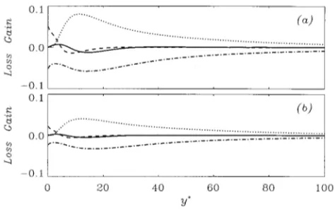
One of the main purposes of SGS models is to dissipate the correct overall amount of energy from the resolved scales. The total energy drain is the negative of the integral, over the wall-normal direction, of the ~time- and plane-averaged!production of SGS energy. The time development of this quantity, together with the integral of the large-scale production, is shown in Fig. 6~b!; in Fig. 6~a!the integral of the large-scale and SGS energy is shown. Under the time-dependent normalization (u_t and n) the subgrid-scale pro-duction and energy do not vary as much as when they are normalized by the initial u_t and n, indicating that they are better described by the local state of the turbulence; by con-trast, the large-scale quantities vary less when normalized by the initial friction velocity and viscosity.

In Fig. 7 profiles of2«sgs are compared with those

ob-tained from several models. The Smagorinsky model not only provides excessive levels of the production throughout the channel, but also does not predict accurately the increase in production that follows the imposition of the perturbation. The time development of the production of SGS energy in-tegrated over the channel height is shown Fig. 8; the integral normalized by its initial value @Fig. 8~a!# indicates that the scale-similar models8,9 and the dynamic model6,7follow the trend more closely. The unnormalized values@shown in Fig. 8~b!#indicate that the scale-similar models tend to underpre-dict the production of SGS energy, consistent with the find-ings of Bardina et al.,8 who developed the mixed model, which includes a dissipative as well as a scale-similar part, to overcome this shortcoming.

FIG. 5. Production of SGS and large-scale energy, normalized by u_tand n. Accelerating channel flow, tophat filter, Di52Dxi. ,

tut,o/d50.06; - - - -, tut,o/d50.32; - • -•-•, tut,o/d50.52;• • • •,

tu_t,o/d50.70.~a!Production of SGS energy;~b!production of large-scale energy.

FIG. 6. Time development of the integral of the large-scale and SGS quan-tities normalized by their initial values. Accelerating channel flow. Tophat filter,Di52Dxi. Lines without symbols: quantities normalized by ut,oand no; lines with symbols: quantities normalized by utandn.~a! , Large-scale energy; - - - -, SGS energy.~b! , Production of large-scale

en-ergy; - - - -, production of SGS energy.

FIG. 7. Wall–normal distribution of the exact and modeled production of SGS energy, normalized by ut,oandno. Accelerating channel flow. Tophat filter, Di52Dxi. n Exact; , dynamic eddy viscosity model;

6,7

- - - -, Smagorinsky model1_@Eq.~8!#;

-•-•-•, scale similar model;9

• • • •, scale similar model.8_~a!tu

t,o/d50;~b!tut,o/d50.13;~c!tut,o/d50.32.

FIG. 8. Time development of the integral of the production of SGS energy. Accelerating channel flow. Tophat filter; Di52Dxi. nExact; , dy-namic eddy viscosity model;6,7 _{- - - -, Smagorinsky model}1 _{@Eq. ~ 8!#;} -•-•-•, scale similar model;9

The increased production predicted by the Smagorinsky model is particularly significant in the near-wall layer, where the scale-similar and dynamic models predict the response to the perturbation fairly accurately~Fig. 9!. In the buffer layer and above the perturbation does not appear to have such a strong effect.

The principal shortcoming of eddy-viscosity models is the fact that the time scale,u¯Su21, is mostly affected by the

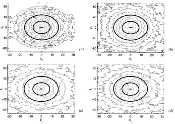
large scales; thus they do not, in general, respond well to perturbations that affect mostly the small scales. This is the reason for the poor performance of the Smagorinsky model in this flow. The dynamic eddy-viscosity model appears to compensate for this deficiency by adjusting the model coef-ficient according to the state of the smallest resolved scales; the scale-similar models have a similar behavior. This is evi-denced in Fig. 10, in which the development of the kinetic energy spectrum at y1513 is shown. The increase in energy at the high wave numbers is apparent. The scales that con-tribute most to the resolved turbulent stressesLi j ~to a first

approximation, the wave numbers contained between the two ellipses in the figure! also increase significantly during the transient, more so than the largest scales of motion~the con-tours near the origin!, which remain essentially unchanged. Thus it appears that the double filtering operation employed by both dynamic and scale-similar models is beneficial in isolating the scales that most closely represent the smallest scales of motion.

C. Three-dimensional boundary layer

Similar results were obtained from the three-dimensional boundary layer simulation. In this flow the perturbation is applied more gradually, and is also localized in space~at the wall!, while the Reynolds number change of the previous flow is felt everywhere. The SGS energy ~Fig. 11! can be observed to react more quickly to the imposition of the per-turbation than the large-scale energy ~especially near the wall!, but the phenomenon is not as clear as in the preceding case, due to the local nature of the perturbation.

The more accurate predictions obtained by the dynamic and scale-similar models are evidenced in Figs. 12 and Figs. FIG. 9. Time development of exact and modeled production of SGS energy.

Accelerating channel flow. Tophat filter,Di52Dxi. All quantities are nor-malized by u_t,oandn, and their initial value.nExact; , dynamic eddy viscosity model;6,7_{- - - -, Smagorinsky model}1_@Eq.~8!#;

-•-•-•scale simi-lar model;9

• • • •, scale similar model.8 _{~a! y}1_{58; ~b! y}1_{513; ~c!}

y1531;~d!y15110.

FIG. 10. Kinetic energy spectra~normalized by ut,o) at y1513. Accelerating channel flow. The contour levels are exponentially spaced between 1027~black! and 100_{~grey!; the two ellipses roughly correspond to the grid- and test-filter wave numbers.~a!tu}

t,o/d50;~b!tut,o/d50.13; ~c!tut,o/d50.32;~d!

13, in which, respectively, the integrated production of SGS energy, 2«_sgs, and its development at several wall-normal locations are shown. The Smagorinsky model initially pre-dicts increased production in the near-wall region~instead of the reduced dissipation that is observed in the DNS data!, reflecting the imposition of the transverse shear ]W/]y , which gives an increase in the eddy viscosity. The other models follow the correct trend, because the smallest re-solved scales are used to evaluate the coefficient. This is confirmed by the kinetic energy spectra ~Fig. 14!, which show features similar to those observed in the accelerating channel flow. The scales included between the two filters behave in a manner very similar to the unresolved scales.

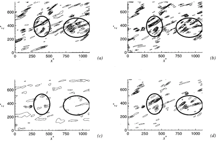
Another useful feature of scale-similar models is that they parametrize the unresolved scales in terms of the small-est resolved ones, which have been shown15–17to be respon-sible for most of the energy transfer between resolved and unresolved scales. Piomelli and co-workers12 observed sig-nificant correlation between regions of high Reynolds stress and production of SGS energy. This correlation can be ob-served in the present data as well. Figure 15 compares con-tours of total production and production of SGS energy. A strong correlation can be observed between the exact

2«sgsand the total production; this correlation is reproduced

well by the scale-similar model, but less accurately by the eddy viscosity model, which, being statistical in nature, can-not be expected to be as successful in reproducing determin-istic events of the type responsible for the distribution of

2«sgs.

IV. CONCLUSIONS

The velocity fields obtained from the direct simulation of two nonequilibrium flows, an accelerating channel flow and a three-dimensional boundary layer, were studied to deter-mine the response to perturbations of the subgrid scales of motion, and their return to equilibrium.

The subgrid scales have a reduced turnover time com-pared with the resolved scales of motion. The fact that this time-scale is not a small fraction of the large-eddy turnover time is partly due to the low Reynolds number of the DNS data used in the present a priori study; in such situations, the strongest interactions between resolved and unresolved scales occur between structures within two octaves of the cutoff wave number. At high Reynolds numbers, when widely separated scales are present, this local interaction may be less dominant, but is still expected to be relevant.

In both flows under consideration, equilibrium turbu-lence is perturbed, and a new equilibrium is reached. In both cases the subgrid scales reach the new equilibrium substan-tially faster than the large, resolved, ones. However, the re-turn to equilibrium of the subgrid scales requires a finite time and is not instantaneous.

From a modeling point of view, this result indicates that SGS models would benefit from incorporating nonequilib-rium behavior to predict more accurately engineering flows, in which a variety of effects ~pressure gradients, secondary shear, etc.! may act to perturb the canonical flows. An effi-FIG. 11. SGS and large-scale energy, normalized by ut,o.

Three-dimensional boundary layer. Tophat filter, Di52Dxi. , tut,o/d50; - - - -, tu_t,o/d50.075; -•-•-•, tut,o/d50.15;• • • •, tut,o/d50.30, —

•••—, tu_t,o/d50.75.~a!SGS energy;~b!large-scale energy.

FIG. 12. Time development of the integral of the production of SGS energy. Three-dimensional boundary layer. Tophat filter,Di52Dxi. All quantities are normalized by ut,oandn, and their initial value.nExact; , dynamic eddy viscosity model;6,7_{- - - -, Smagorinsky model}1_@Eq.~8!#;

-•-•-•, scale similar model;9

• • • •, scale similar model.8

FIG. 13. Time development of exact and modeled production of SGS en-ergy. Three-dimensional boundary layer. Tophat filter,Di52Dxi. All quan-tities are normalized by ut,oandn, and their initial value.nExact; , dynamic eddy viscosity model;6,7 _{- - - -, Smagorinsky model}1 _{@Eq. ~8!#;} -•-•-•, scale similar model;9• • • •, scale similar model.8~a!y158;~b!

cient and inexpensive way to take those effects into account is to use the smallest resolved scales to parametrize the un-resolved ones, as is done in scale-similar and dynamic mod-els. These models have been found to respond more accu-rately to perturbations than models, like the Smagorinsky model, that are mostly affected by the largest scales of

mo-tion. The present results further confirm the robustness of dynamic SGS models in computing nonequilibrium flows.

While the dynamic eddy viscosity model predicts the overall levels of energy drained from the large scales quite accurately, scale-similar models are much more effective at representing the correlation between the production of large-FIG. 14. Kinetic energy spectra ~normalized by ut) at y1515. Three-dimensional boundary layer. The contour levels are exponentially spaced between 1027 _{~black! and 10}0 _{~grey!; the two ellipses roughly correspond to the grid- and test-filter wave numbers. ~a! tu}

t,o/d50; ~b! tut,o/d50.14; ~c!

tu_t,o/d50.29;~d!tut,o/d50.60.

scale energy and production of SGS energy that has been observed in these nonequilibrium flows, and also in the near-wall region of equilibrium boundary layers.12Mixed models, which combine a scale-similar model with a dissipative, eddy-viscosity term, are likely to be very effective parametri-zations of the SGS stresses in nonequilibrium flows.

ACKNOWLEDGMENTS

Support for this research was provided by the Office of Naval Research, Grants No. N00014-91-J-1638 ~UP! and No. N0014-94-1-0016 ~GNC and JK! monitored by Dr. L. Patrick Purtell. Computer time was provided by the Naval Oceanographic Office, the NAS program at NASA–Ames Research Center, and the San Diego Supercomputer Center.

1_{J. Smagorinsky, ‘‘General circulation experiments with the primitive} equations. I. The basic experiment,’’ Mon. Weather Rev. 91, 99~1963!. 2_{D. K. Lilly, ‘‘The representation of small-scale turbulence in numerical}

simulation experiments,’’ Proceedings of the IBM Scientific Computing

Symposium on Environmental Sciences, Yorktown Heights, NY~ unpub-lished!.

3_{L. M. Smith and V. Yakhot, ‘‘Short and long-time behavior of eddy} vis-cosity models,’’ Theor. Comput. Fluid Dyn. 4, 197~1993!.

4

J. Bardina, J. H. Ferziger, and R. S. Rogallo, ‘‘Effect of rotation on iso-tropic turbulence: Computation and modelling.’’ J. Fluid Mech. 154, 321 ~1985!.

5_{G. N. Coleman, J. Kim, and A.-T. Le, ‘‘A numerical study of}

three-dimensional boundary layers,’’ Proceedings of the 10th Turbulent Shear

Flow Conference, State College, PA, 1995~unpublished!.

6_{M. Germano, U. Piomelli, P. Moin, and W. H. Cabot, ‘‘A dynamic} subgrid-scale eddy viscosity model,’’ Phys. Fluids A 3, 1760~1991!. 7_{D. K. Lilly, ‘‘A proposed modification of the Germano subgrid-scale}

clo-sure method,’’ Phys. Fluids A 4, 633~1992!. 8

J. Bardina, J. H. Ferziger, and W. C. Reynolds, ‘‘Improved subgrid scale models for large eddy simulation,’’ AIAA Paper No. 80–1357, 1980. 9

S. Liu, C. Meneveau, and J. Katz, ‘‘On the properties of similarity subgrid-scale models as deduced from measurements in a turbulent jet,’’ J. Fluid Mech. 275, 83~1994!.

10

E. R. Van Driest, ‘‘On the turbulent flow near a wall,’’ J. Aero. Sci. 23, 1007~1956!.

11

U. Piomelli, ‘‘High Reynolds number calculations using the dynamic subgrid-scale stress model,’’ Phys. Fluids A 5, 1484~1993!.

12_{U. Piomelli, Y. Yu, and R. J. Adrian, ‘‘Subgrid-scale energy transfer and} near-wall turbulence structure,’’ Phys. Fluids 8, 215~1996!.

13_{J. Kim, P. Moin, and R. D. Moser, ‘‘Turbulence statistics in} fully-developed channel flow at low Reynolds number,’’ J. Fluid Mech. 177, 133~1987!.

14_{N. N. Mansour, J. Kim, and P. Moin, ‘‘Reynolds stress and} dissipation-rate budgets in a turbulent channel flow,’’ J. Fluid Mech. 194, 15~1988!. 15_{R. H. Kraichnan, ‘‘Eddy viscosity in two and three dimensions,’’ J.}

At-mos. Sci. 33, 1521~1976!.

16_{J. A. Domaradzki, W. Liu, and M. E. Brachet, ‘‘An analysis of} subgrid-scale interactions in numerically simulated isotropic turbulence,’’ Phys. Fluids A 5, 1747~1993!.

17