A New Method for Forecasting via Feedback
Control Theory
Manlika Rajchakit,
Member, IAENG
Abstract—In this paper, we present a new method for forecasting time series data. Firstly, we give a brief review of five standard statistical techniques from the literature, namely the ARIMA, Holt’s method, Holt-Winters method, Decomposition method and Regression analysis. Then, we apply feedback control theory to five well-known forecasting methods. By introducing the concept of mean absolute error, different results are obtained and compared via feedback control theory. In summary, the comparison results illustrate that the new method proposed in this paper provides improved forecasting accuracy and significantly decrease the forecasting error than the existing individual forecasting methods.
Index Terms—ARIMA, Holt’s Method, Decomposition Method, Regression Analysis, Feedback Control Theory.
I. INTRODUCTION
Nowadays, people often use forecasting techniques to model and predict economic activities, population growth, stocks, insurance/re-insurance, industrial and science [1]. Over the past decades, several models have been developed for time series forecasting. ARIMA is the method first introduced by Box and Jenkins and until now become the most popular models for forecasting univariate time series data. This model has been originated from the autoregressive model (AR), the moving average model (MA) and the combination of the AR and MA, the ARMA models.
In the case where seasonal components are included in this model, then the model is called as the SARIMA model. Box and Jenkins procedure that contains three main stages to build an ARIMA model, i.e. model identification, model estimation and model checking is usually used for determining the best ARIMA model for certain time series data [2]. Moreover, the exponential smoothing methods of forecasting involve a mix of adaptive levels, growth rates and seasonal effects [3]. The exponential smoothing is an extension of ES designed for trend time series [4]. The Holt-Winters method (triple exponential smoothing) takes into account both seasonal changes and trends. They provide good forecasts with imply formulations, allowing the incorporation of error, trend and seasonal component in a comprehensive manner [5-9]. Furthermore, time series regression basically relates the dependent variable to functions of time describing trend and seasonal component. It is most profitably used when the components describing the time series to be forecast remain constant overtime [10] and it application by many researchers in many areas [11-14]. Additionally, decomposition models to forecast time series that exhibit trend and seasonal effects. These models have been found
Manuscript received November 02, 2016; revised December 25, 2016. This work was supported in part by Faculty of Science Maejo University, and The Office of Agricultural Research and Extension Maejo University Thailand.
Manlika Rajchakit is with the Department of Statistics, Maejo University, Chiang Mai 50290, Thailand e-mail: [email protected].
useful when the parameters describing a time series are not changing over time [10]. There are a number of papers in the literature which deal with the extrapolation of time series through the extrapolation of individual components. However, in all applications of the classical decomposition technique, the residual component after the elimination of any trend, cyclical and seasonal variations is always assumed to be a random variable with a constant variance, and is therefore exclude from the forecasting process [15]. Then, we apply feedback control theory to five well-known fore-casting methods. Moreover, we demonstrate an illustrative example of these methods with real data set and compare different results via feedback control theory by introducing the concept of mean absolute error (MAE).
In this paper, a new forecasting method is developed via feedback control theory with application to real data set. The five forecasting methods namely the ARIMA, Holt’s method, Holt-Winters method, Decomposition method and Regression analysis are included in the analysis and can be implemented readily in a software package. The statistical software used in this paper are SPSS and Minitab.
In the following section, we review the five modeling approaches to time series forecasting and we prefer the time series via feedback control theory. Empirical results for comparing the forecasting techniques from five real data set are illustrated in Section 3. The final section provides the conclusion.
II. METHODOLOGY
In this paper, we focus on the basic principles and modeling process of the ARIMA, Exponential smoothing, Decomposition and Regression analysis.
2.1 The ARIMA Model [10]:
Classical Box-Jenkins models are describe thestationary
time series. A time series is stationary if the statistical properties (for instance, the mean and the variance) of time series are essentially constant through time. If n-number of values seem to fluctuate with constant variation around a constant meanµ, then it is reasonable to believe that the time series is stationary. If the n values do not fluctuate around the constant mean or do not fluctuate with constant variation, then it is reasonable to believe that the time series is nonsta-tionary. In this paper, we consider only nonstationary time series. In this case where the data have trend component, we call an autoregressive integrated moving average or ARIMA
series data[16]. Hence an ARIMA(p, d, q)can be written as
ˆ
yt=θ0+ϕ1yt−1+ϕ2yt−2+. . .+ϕpyt−p
+εt−θ1εt−1−θ2εt−2−. . .−θqεt−q,
Moreover, the SARIMA (P, D, Q)m can be written as
ˆ
yt=θ0+φ1yt−m+φ2yt−2m+. . .
+φPyt−P m+εt−ω1εt−m
−ω2εt−2m−. . .−ωQεt−Qm.
Therefore a more general seasonal ARIMA model orders
(p, d, q)×(P, D, Q)m with period m is
Φ∗(Bs)Φ(B)(1−B)d(1−Bm)Dyˆt =δ+ Θ∗(Bm) Θ(B)εt,
ˆ
yt=θ0+ϕ1yt−1+ϕ2yt−2+. . .+ϕpyt−p
+εt−θ1εt−1−θ2εt−2−. . .−θqεt−q +φ1yt−m+φ2yt−2m+. . .+φPyt−P m
−ω1εt−m−ω2εt−2m−. . .−ωQεt−Qm.
where
yt is the actual value at time period t.
p, d, q are the autoregressive, differencing and moving average term in the ARIMA model.
P, D, Q are the autoregressive, differencing and moving average term for the seasonal part of ARIMA model.
ϕi, θj are model parameters for ARIMA term order p
andqrespectivelyi= 1,2, . . . , pandj= 1,2, . . . , q.
φi, ωj are model parameters for SARIMA term orderP
andQrespectively;i= 1,2, . . . , P andj= 1,2, . . . , Q.
εt are random errors which assumed to be independently
and identically distributed with a mean of zero and a constant variance ofσ2 [17].
m are the period of seasonal (for example weekly, monthly and quarterly).
2.2 Exponential Smoothing Technique [10]:
Exponential smoothing provides a forecasting method that is most effective when the components (trend and seasonal factors) of the time series may be changing over time. Simple exponential smoothing is suitable method for time series has no trend. While, Holt’s method is appropriate when both the level (ℓt) and the growth rate
(bt) are changing. Furthermore, Holt-Winter methods are exponential smoothing procedures for seasonal data.
2.2.1 Holt’s Method:
A point forecast made in time period t for yˆt+τ isyˆt+τ = ℓt+τ bt (τ= 1,2, . . .). The smoothing equations are as
followℓt=αyt+(1−α) [ℓt−1+bt−1], bt=γ[ℓt−ℓt−1]+
(1−γ)bt−1.
2.2.2 Holt-Winters Method:
Holt-Winters method is designed for time series that ex-hibit linear trend at least locally. The additive Holt-Winters method is used for time series with constant (additive) seasonal variation, whereas the multiplicative Holt-Winters method is used for time series with increasing (multiplica-tive) seasonal variation.
2.2.3 Additive Holt-Winters Method
A point forecast made in time periodt foryˆt+τ is
ˆ
yt+τ(t) =lt+τ bt+snt+τ−m, (τ= 1,2, . . .).
The smoothing equations are given by
ℓt=α(yt−snt−m) + (1−α) [ℓt−1+bt−1],
bt=γ[ℓt−ℓt−1] + (1−γ)bt−1,
snt=δ[yt−ℓt] + (1−δ)snt−m. 2.2.4 Multiplicative Holt-Winters Method
A point forecast made in time periodt foryˆt+τ is
ˆ
yt+τ(t) = (lt+τ bt)snt+τ−m, (τ= 1,2, . . .).
The smoothing equations are given by
ℓt=α(yt/snt−m) + (1−α) [ℓt−1+bt−1],
bt=γ[ℓt−ℓt−1] + (1−γ)bt−1,
snt=δ[yt/ℓt] + (1−δ)snt−m.
where
ℓt is estimated for the level . bt is estimated for the growth rate.
snt is estimated for the seasonal factor of the time
series in time series periodt.
snt+τ−m is the ”most recent” estimate of the seasonal
factor for the reason corresponding to time periodt+τ.
α, γ, δ are the smoothing constants between0 and1.
ℓt−1, bt−1 are estimates in time period t−1 for the level and growth rate.
snt−m is the estimate in time period t−m for the
seasonal factor.
m is the period of the seasonality.
τ is the τ-step-ahead forecast.
2.3 Decomposition Method [10]:
The basic idea behind these models is to decompose the time series into several factors: trend, seasonal, cyclical and irregular (error). Multiplicative decomposition appropriate for a time series that exhibits increasing or decreasing seasonal variation. When the parameters describing the series are not changing over time. Whereas, Additive decomposition found useful when a time series that exhibits constant seasonal variation. The multiplicative decomposition model is
Yt=T Rt×SNt×CLt×IRt
The additive decomposition model is
Yt=T Rt×SNt+CLt+IRt
where
Yt are the observed value of the time series in time
periodt.
T Rt are trend component (or factor) in time period t. SNtare seasonal component (or factor) in time periodt. CLtare cyclical component (or factor) in time periodt. IRtare irregular component (or factor) in time periodt.
The estimates trt, snt, clt and irt are generally used to
and cycle component, we assume T Rt and CLt to equal
zero. The point forecast for the multiplicative decomposition model is
ˆ
yt=trt×snt.
The point forecast for the additive decomposition model is
ˆ
yt=trt+snt.
2.4 Regression Analysis [18]:
Regression analysis is a statistical technique for modeling and investigating the relationships between an outcome or response variable and one or more predictor or regression variables. The end result of a regression analysis study is often to generate a model that can be used to forecast or predict future values of the response variable given specified values of the predictor variable.The simple linear regression model involves a single predictor variable,which can be written as
y=β0+β1x+ε,
where
y is the response.
x is the predictor variable.
β0, β1 are unknown parameters.
ε is an error term.
The model parameters or regression coefficients β0 and
β1 have a physical interpretation as the intercept and the slope of a straight line, respectively. The slopeβ1 measures the change in the mean of the response variable yt for a
unit change in the predictor variable x. These parameters are typically unknown and must be estimated from a sample of data. The error termεaccounts for deviations of the actual data from the straight line specified by the model equation. We usually think of ε as a statistical error, so we define it as a random variable and will make some assumptions about its distribution. For example, we typically assume that
ε is normally distributed with mean zero and variance σ2, abbreviated asN(0, σ2).
Note that the variance is assumed to be constant; that is, it does not depend on the value of the predictor variable (or any other variable).
Additionally, [10] one useful from of the linear regression model is what we call the quadratic regression model. The quadratic regression model relatingytoxis
y=β0+β1x1+β2x2+ε.
Then, we apply regression analysis to time series analysis. The simple linear regression is as follow
ˆ
yt=b0+b1t.
The quadratic regression model is
ˆ
yt=b0+b1t+b2t2.
whereb0, b1are estimated using the method of least squares of the unknown parameter β0 andβ1 respectively.
2.5 Time Series with Feedback Control Theory/
The Feedback Control Methodology
Striking developments have taken place since 1990 in feedback control theory [19]. The subject has become both more rigorous and more applicable. The rigorous is not for its own sake, but rather that even in an engineering discipline rigorous can lead to clarity and to methodical solutions to problems. The applicability is a consequence both of new problem formulations and new mathematical solutions to these problems [20-22]. Moreover, computers and software have changed the way engineering design is done. These developments suggest a fresh presentation of the subject, one that exploits these new developments while emphasizing their connection with classical control. Control systems are designed so that certain designated signals, such as tracking errors and actuator inputs, do not exceed pre-specified levels. Hindering the achievement of this goal are uncertainty about the plant to be controlled (the mathematical models that we use in representing real physical systems are idealizations) and errors in measuring signals (sensors can measure signals only to a certain accuracy). Despite the seemingly obvious requirement of bringing plant uncertainty explicitly into control problems, it was only in the early 1990s that control researchers re-established the link to the classical work of Bode and others by formulating a tractable mathematical notion of uncertainty in an input-output framework and developing rigorous mathematical techniques to cope with it.This formulates a precise problem, called the robust performance problem, with the goal of achieving specified signal levels in the face of plant uncertainty.
Without control systems there could be no manufactur-ing, no vehicles, no computers, no regulated environment-in short, no technology. Control systems are what make machines, in the broadest sense of the term, function as intended. Control systems are most often based on the principle of feedback, whereby the signal to be controlled is compared to a desired reference signal and the discrepancy used to compute corrective control action. Consider the Time series with Feedback Control Theory/The Feedback control methodology:
ˆ
yt=g(yt) +u(t),
where
ˆ
yt is predicted value.
u(t) is feedback control input.It is defined byu(t) =
median error.
Model Selection
error results are reported here. The expressions is depicted below
M AE= n
∑
t=1
|yt−yˆt|/n,
where
yt is the actual value at time t. ˆ
yt is the forecast value at timet. n is the number of observations.
III. EMPIRICALRESULTS
Five real data sets-the expert value of apple juice, the average gold prices (US dollar /oz), the number of tourist arrivals to Thailand by nationality (America), the foreign workers in Thailand, and the influenza patient numbers in Thailand-are considered in this paper to illustrate the effectiveness of the control theory. Each data set is divided into two samples of training and testing. The actual data sets are as follows
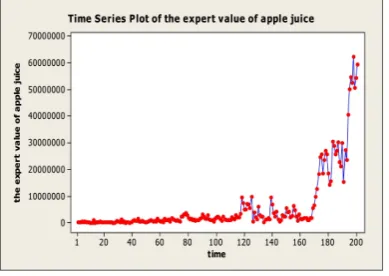
Example 1. The Expert Value of Apple Juice Cases
We considered all monthly series between January 1998 - September 2014, total 201 observations.We divided the data into two groups, the first group used a 16-year data set from January 1998 to December 2013, giving a total of 192 observations as the training data. The second group used 9 observations between January to September in 2014 to finding suitable methods. The time series plot are shown in
[image:4.595.327.525.53.192.2]Fig.1
Fig. 1. The expert value of apple juice series from January 1998 to September 2014.
It is noted that the expert value of apple juice series from Office of Agricultural Economics Ministry remained stable obviously being 1,005,632 baht. After that, the plot grew dramatically being from 9,544,905 to 59,666,747 baht.
Example 2. The Average Gold Prices (US Dollar/Oz)Cases
The last 10 observations is not be used to compute the forecast but to evaluate their accuracy. The plot is shown in
[image:4.595.326.527.383.525.2]Fig.2
Fig. 2. The average gold prices (US dollar/oz) between January 2007 and October 2015.
It is noted that the time plot of the average gold prices from gold traders association reached to the peak obviously 1,780 (US dollar/oz), then the graph declined slightly.
Example 3. The Number of Tourist Arrivals to Thailand by Nationality (America).
The last 9 observations is not be used to calculate the forecast but to evaluate their accuracy. The plot is shown in
Fig.3
Fig. 3. American tourist visitor in Thailand via Suvarnabhumi airport from January 2007 until September 2015.
The time series plot of the number of oversea visitor’s arrivals to Thailand by nationality (America) from department of tourism reveals a periodicity of approximately 9 years.
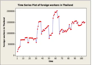
Example 4. The Foreign Workers in Thailand
[image:4.595.74.269.422.560.2]Fig. 4. The foreign workers in Thailand from January 2007 until September 2015.
The plot of the foreign workers in Thailand from office of Foreign Workers Administration shows various changing turning points in the series.
Example 5. The Number of Influenza Patients in Thailand
[image:5.595.73.269.55.193.2]Time plot of the number of influenza patients in Thailand are presented inFig.5
Fig. 5. Quarterly total influenza patients in Thailand, 2003-2015.
The number of influenza patients in Thailand from social and quality of life data base system reveals remained stable for 6 years and then the plot provided a periodicity of approximately 7 years.
Table I. The results of mean absolute error (MAE) obtained using well known time series models with application to feedback control theory
TABLE I
COMPARISONSMAEVALUES OF VARIOUS METHODS WITH APPLICATION TO FEEDBACK CONTROL THEORY OBTAINED FROM
DIFFERENT DATA SETS.
IV. CONCLUSION
Time series analysis is one of the very demanding sub-jects over the last few decades, since can be applied for financial, economic, engineering and scientific modeling. The five other standard statistical techniques from the literature, namely the ARIMA,Holt’s method, Holt-Winters method, Decomposition method and Regression analysis are well known for many researchers. The aim of this research is prefer a new method for forecasting via feedback control theory with application to several non-stationary real data sets. The performance evaluation results indicated that this method can perform well. As it is clear that the errors measures are decline all of cases. Future work can include stationary data and apply adaptive control theory to time series analysis.
REFERENCES
[1] T.A. Jilani and S.M.A. Bomey. (2008) Multivariate stochastic fuzzy forecasting models. Expert Systems with Applications. 35(3): 691-700. [2] Suhartono. (2011). Time series forecasting by using seasonal autore-gressive integrated moving average: subset, Multiplication or Additive model. Journal of Mathematics and Statistics. 7(1): 20-27.
[3] A.N. Beaument. (2014). Data transforms with exponential smoothing methods of forecasting. International Journal of Forecasting. 30(4): 918-927.
[4] C.C.Holt. (2004). Forecasting seasonal and trends by exponentially weighted moving average. International Journal of Forecasting. 20:5-10.
[5] L.Wo, S.Liu and Y.Yang. (2016). Grey double exponential smoothing model and its application on pig price forecasting in china. Applied Soft Computing. 39: 117-123.
[image:5.595.71.271.356.498.2][7] G. Sudheer and A. Suseelatha. (2015). Short term load forecasting using wavelet transform combined with Holt and Winters and weighted nearest neighbour models. International Journal of Electrical Power and Energy Systems. 64: 340-346.
[8] W. Romeijnders, R. Teunter and W.V. Jaarsveld. (2012). A two-step method for forecasting spare parts demand using information on com-ponent repairs. European Journal of Operational Research. 220(2):386-393.
[9] G.Li, Z. Cai, X. Kang, Z.Wu and Y.Wang. (2014).ESPSA: a predication algorithm for streaming time series segmentation. Expert Systems with Application. 41 (14): 6098-6105.
[10] B.L.Bowerman, R.O’Connell and A.Kochler. (2005). Forecasting, Time series and Regression, 4th ed, Thomson Learning, Inc. [11] J. Woody. (2015). Time series regression with persistent level shifts.
Statistics and Probability Letters. 102: 22-29.
[12] A.Azizi, A.Y.Ali, L.W.Ping and M. Mohammadzadeh. (2012). A Hybrid model of ARIMA and Multiple polynomial regression for uncertainties modeling of a serial production line. World Academy of Science, Engineering and technology. 6: 56-61.
[13] Z. Ismail, A. Yahya and A. Shabri. (2009). Forecasting gold prices using multiple linear regression method. American Journal of Applied Science 6(8): 1509-1514.
[14] Recep Duzgun. (2010). Generalized regression neural networks for inflation forecasting. International Research Journal of Finance and Economics. 51: 59-70.
[15] Marina Theodosiou. (2011). Forecasting monthly and quarterly time series using STL decomposition. International Journal of Forecasting. 27:1178-1195.
[16] Suhartono.(2011) . Time series forecasting by using seasonal autore-gressive integrated moving average: subset, multiplicative or additive model. Journal of Mathematics and Statistics 7(1): 20-27.
[17] Peter Zang. (2003). Time series forecasting using hybrid ARIMA and neural network model. Neurocomputing 50: 159-175.
[18] D.C.Montgomery, C. L. Jennings and M. Kulahci. (2008). Introduction to Time Series Analysis and Forecasting. A John Wiley and SONS, Inc.,Publication
[19] J. Doyle, B. Francis and A. Tannenbaum (1990). Feedback Control Theory,.Macmillan Publishing Co.,
[20] V. N. Phat and K. Ratchagit. (2011). Stability and stabilization of switched linear discrete-time systems with interval time-varying delay. Nonlinear Analysis: Hybrid Systems. 5 : 605-612.
[21] V. N. Phat, Y. Khongtham and K. Ratchagit (2012). LMI approach to exponential stability of linear systems with interval time-varying delays, Linear Algebra and its Applications. 436:243-251.
[22] K. Ratchagit. (2007). Asymptotic stability of delay-difference system of Hopfield neural networks via matrix inequalities and application. International Journal of Neural Systems. 17: 425-430.