Spatial Heterogeneity of Surface Roughness
on Tilled Loess Slopes in Erosion Stages
Qingfeng ZHANG*, Jian WANG and Faqi WU
Northwest A&F University, Yangling, P.R. China
*Corresponding author: [email protected]
Abstract
Zhang Q., Wang J., Wu F. (2018): Spatial heterogeneity of surface roughness on tilled loess slopes in erosion stages. Soil & Water Res., 13: 90−97.
The main soil erosion areas of the Chinese Loess Plateau are tilled slopes. The knowledge of their spatial hetero-geneity will contribute to the understanding of erosion mechanisms on a microtopographic scale. In this study, the spatial heterogeneity of four conventionally tilled slopes was examined under simulated rainfall conditions using a semivariogram-based methodological framework. Results show that all tilled slopes have a relatively stable spatial structure and the erosion stages of all tilled slopes have a similar spatial variability. The rainfall in the splash, sheet, and rill erosion stages has a degree of relief effect, strengthening effect, and relief effect on the surface roughness, respectively. However, the effects of tillage practices and slope gradient on the spatial heterogeneity are much larger than those of the rainfall. The spatial heterogeneity decreases with increasing slope gradient. The general autocor-relation scale of the tilled slopes is 3.15 m and their fractal dimension ranges from 1.59 to 1.85. The tilled slopes have certain anisotropy with respect to the slope direction from 10° to 22.5° while they show isotropy or weaker anisotropy in other directions. In this work, a semivariogram-based methodological framework was established for the spatial heterogeneity of microtopographic-scale slopes. The results also provide a theoretical foundation for future tillage measures on sloping fields of the Loess Plateau.
Keywords: erosion effect; semivariogram; surface roughness; tillage measures
Abbreviations: SH – spatial heterogeneity; BP – backhoe ploughing; CT – contour tillage; DP – digging ploughing;
RL – rake levelling; E30 – 30-minute rainfall intensity; BR – before rainfall, original slopes were prepared for rainfall; SpE – splash erosion, the phase prior to the runoff initiation; ShE – sheet erosion, the phase defined by the appearance of fish scale-shaped pits and small-scale overfall; RE – rill erosion, the phase during which fish scale-shaped pits and overfall form the rill; r(h) – semivariance (mm2); Z(x) – elevation at location x (mm); h – lag distance between the sam-pling points (mm); N(h) – number of data pairs; C + C0 – sill of the variogram, overall maximum spatial variability in a system (mm2); a – codomain or range of the variogram (mm); C – structural variance, which reflects the spatial variability due to spatial structure properties (mm2); C
0 – nugget variance, which reflects the spatial variability due to random ele-ments (mm2); C/(C + C
0) – base effect; Fa – anisotropy ratio = a2/a1; a2 – the largest range of the model describing the semivariance function in the θ direction; a1 – the range of the model describing the semivariance function toward lower spatial continuity θ + 90°; m – slope of the double logarithmic semivariogram; D – fractal dimension used to describe the overall complexity; SD – spatial dependence
The Chinese Loess Plateau has long been suffering from serious soil erosion issues. The soil erosion of tilled sloping land is estimated to contribute 50–60% of the total soil erosion of the Loess Plateau (Wei
et al. 2006).
The soil surface roughness, which reflects the mi-crovariation of surface-relative elevations, has been
Soil & Water Res., 13, 2018 (2): 90–97 Original Paper
https://doi.org/10.17221/130/2017-SWR
basic questions are common and need to be addressed when studying the SH of surface roughness: (1) How does the variability alter depending on the sampling distance?; (2) What part and which factor (random and structural factors) contribute more to the spatial variability?; and (3) What is the specific slope direc-tion of the variability? Many studies highlighted the hydraulic characteristics and dynamic mechanisms and randomness and complexity of the surface roughness in the past (e.g., Römkens & Wang 1984; Shen et al.
2016). However, there are few detailed studies on the SH of surface roughness in erosive stages, which affects the in-depth understanding of erosion mechanisms, especially on the microtopographic scale. Therefore, the objective of this study was to examine the SH of four typical tilled slopes under simulated rainfall conditions.
MATERIAL AND METHODS
Experimental materials. The sample soil used in this study was collected from a plough layer in Yangling in the Shaanxi Province, which is located at the southern edge of the Chinese Loess Plateau (107.56°–108.08°E, 34.14°–34.20°N). The “loutu” soil, classified as an Earth-cumuli-Orthic Anthrosol (USDA Taxonomy) or Anthrosols (AT) (WRB, 2014), is grey-brown, loose, and granular and contains silty and clayey soil particles.
Preparation of the soil tank.The sample soil was air-dried, gently crushed, sieved through a 10-mm sieve, and filled in ten 10-cm layers into soil tanks (100 × 200 cm2) to a depth of 100 cm. Before packing the soil
tanks, the soil water content was determined and used to calculate how much soil was needed for each soil layer to obtain the target bulk density (1.30 g/cm3).
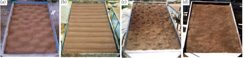
Five slope gradients of 9% (5°), 18% (10°), 27% (15°), 36% (20°), and 47% (25°) typical of the Loess Plateau were designed and prepared when the soil tanks were completely packed. Four traditional Loess Plateau tillage measures were imposed on the sloping surface such as
backhoe ploughing (BP), contour tillage (CT), digging ploughing (DP), and rake levelling (RL; Figure 1). Sub-sequently, all soil tanks were allowed to settle for 48 h.
Before the runs, all soil slopes were subjected to pre-rain with a rainfall intensity of 30 mm/h until surface flow occurred. The purpose of pre-rain was to maintain consistent soil moisture content, which was gravimetrically adjusted to 10 g/100 g, and con-solidate loose soil particles (Shen et al. 2016).
Experimental procedures.In Yangling, the maxi-mum 30-minute rainfall intensity is expected to occur once per 100 years and reaches up to 120.85 mm/h. Hence, the experimental rainfall intensity in this study was set to 2.0 mm/min(i.e., 120 mm/h).
A down-sprinkler rainfall simulator system (Zheng & Zhao 2004) was used to apply rainfall (Zhou & Shangguan 2007). Three successive rainfall events were employed during four erosion processes: before rainfall (BR), splash erosion (SpE), sheet erosion (ShE), and rill erosion (RE). The first and second rainfall events had ~25-min duration; the third rainfall event lasted ~35 min.
A laser rangefinder (Zhang et al. 2014) was used for the automated measurement of the point-by-point elevation in a regularly spaced grid (2 × 2 cm).
Data analysis
Semivariogram. A semivariogram was used to characterize the variability of the surface roughness between data points (Pandey & Pandey 2010). It is defined as:
(1)
where:
r(h) – semivariance of the point elevation (mm2)
h – lag distance between the points (mm) Z(x) – elevation of the point x (mm)
[image:2.595.98.501.628.724.2]N(h) – number of data pairs
Figure 1. Four traditional tillage measures in the Chinese Loess Plateau listed as: (a) backhoe ploughing (BP), (b) contour tillage (CT), (c) digging ploughing (DP) and (d) rake levelling as the control (RL), established by experienced farmers
( )
2
1
1
( ) [ ( ) ( )]
2 ( )
N h
i i i
r h Z x Z x h
N h
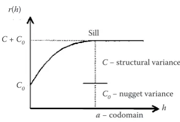
The semivariogram graph (Figure 2) can be de-picted using theoretical models such as spherical, Gaussian, exponential, or linear models. Based on Figure 2, r(h) initially increases with h and reaches a sill (C + C0; mm2) when h is close to the codomain
(a; mm); the sill is the limit of r(h) and is indicative of the overall amplitude of the spatial variability of the point elevation of the soil surface; a is the range or minimum lag distance at which spatial autocorrelation or dependence between the elevation measurements is no longer observed. Therefore, it is a measure of the amplitude of the horizontal variability of the soil surface (Andrés et al. 2015). The structural variance (C; mm2) and nugget variance (C
0; mm2) reflect the SH of the surface roughness, respectively, which is due to spatial constitutive (autocorrelation) properties and randomness elements. The base ef-fect, ratio of C/(C + C0), is indicative of an enhanced variability of > 75%, 25%–75%, and < 25%, indicating strong, moderate, and weak spatial autocorrelation or dependence, respectively.
Geometric anisotropy.The spatial variability of the variables in a system is related to the spatial sampling distance, which often varies with direction (Craw-ford & Hergert 1997). If the spatial dependence structure is only a function of the distance separating the observed locations, the process that describes the spatial variability is isotropic. Conversely, if this structure differs with respect to the direction, the process is anisotropic (Webster 1985). Specifically, geometric anisotropy can be characterized by two parameters, anisotropy angle and ratio. The anisot-ropy angle is the azimuth angle of the direction with greater spatial continuity, which is the angle between the y-axis and the direction with the maximum range. The anisotropy ratio is the ratio between the ranges of the directions with greater and smaller continu-ity, which is the ratio between the maximum and minimum ranges (Fa = a2/a1). Therefore, its value is always greater or equal to one (Guedes et al. 2013). When Fa ≈ 1, the SH of the surface roughness as a whole exhibits an isotropy. An anisotropy exists when
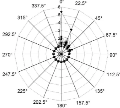
Fa > 1 (Jiang et al. 2010). A greater Fa indicates a stronger spatial variability, while a smaller Fa indi-cates a weaker spatial variability or a stronger spatial autocorrelation. Directional semivariograms can be constructed to preliminarily identify the existence and type of anisotropy (Guedes et al. 2013). In this study, seventeen anisotropy angles were used to vali-date these semivariograms with a tolerance radius of 22.5°, following the system of azimuth direction
measurement, considering true north as direction 0°, and varying the other directions clockwise.
Fractal dimension.The fractal dimension (D) is employed to characterize the SH:
D = 2 – m/2 (2)
where:
m – slope of the double-log semivariogram
If D = 2, the sample surface roughness is homoge-neous or isotropic, which indicates that the elevation points are space-independent. If D = 1, the sample surface roughness distribution is linear, with a gra-dient feature, which means that the surface rough-ness monotonously changes as the sample interval increases (Lü et al. 2006).
RESULTS AND DISCUSSION Overall spatial variation
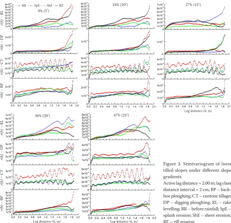
Figure 3 shows a notable trend; r(h) of each slope increases with h and remains relatively stable within a certain sampling scale. Moreover, the same tillage slope exhibits an extremely similar spatial variability, regardless of the slope gradients or erosive stages. This behaviour exemplifies that the surface rough-ness of different tilled slopes has a relatively stable spatial variability. This is the same as the result from Zhang (Zhang et al. 2014).
Variation on different scales. The r(h) of all tilled slopes rises steadily from 0 to 15 cm in different erosion stages (Figure 3), which might be linked to local randomicity factors such as incomplete tillage measure or edge effects of soil tanks. On a larger Figure 2. Generalized semivariogram structure
The semivariance r(h) increases with the lag distance h within the codomain a, and the overall spatial variability will reach the maximum value at the point of codomain, while the spatial autocorrelation or dependence will fade away outside a
r(h)
C + C0
C0
Sill
C − structural variance
Soil & Water Res., 13, 2018 (2): 90–97 Original Paper
https://doi.org/10.17221/130/2017-SWR
scale from 15 to 150 cm, r(h)remains relatively stable, suggesting that the related semivariogram graph can be used to simulate the real surface very well. On the scale of 180–200 cm, on the one hand, r(h) increases rapidly, implying that the total SH increases gradu-ally with the scale. The microtopographic (tillage measure, slope orientation, and slope profile) and rainfall (intensity, duration, amount) characteristics are the predominant factors impacting the surface roughness variation on a larger spatial scale. On the other hand, we also observed a rapid decrease in
r(h), which indicates that the surface roughness does not have a quantitative spatial correlation and lacks defined spatial structures. This behaviour might be caused by local factors such as edge effects.
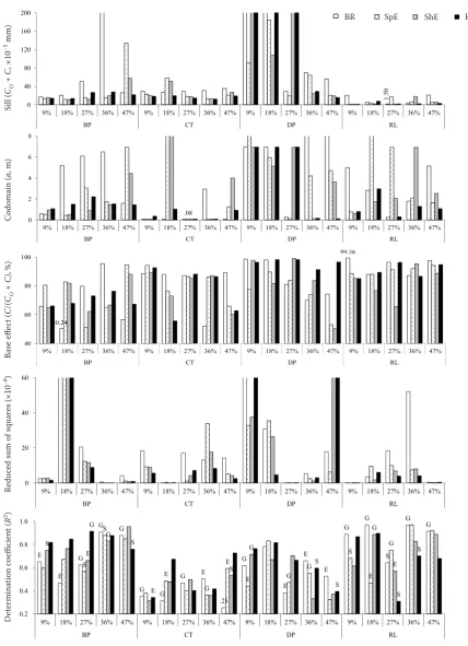
Variations in different erosion stages. During the successive water erosion stages, the overall sill of tilled slopes has the following order: SillBR > SillSpE >
SillRE > SillShE (Figure 4). Correspondingly, the SH or the overall maximum spatial variability is reduced in the splash erosion stage, increased in the sheet erosion stage, and slightly re-reduced in the rill ero-sion stage. This means that the rainfall has a certain relief, strengthening, and relief effect on the surface roughness in the splash, sheet, and rill erosion stages, respectively.In general, the rainfall exerts a gentle force on the surface roughness, which is in accordance with previous works by Zhao et al. (2014).
[image:4.595.64.531.92.543.2]Variations of different slope gradients. Based on the sill of the different slope gradients, the slope of Figure 3. Semivariogram of loess tilled slopes under different slope gradients
Active lag distance = 2.00 m; lag class distance interval = 2 cm; BP – back-hoe ploughing; CT – contour tillage; DP – digging ploughing; RL – rake levelling; BR – before rainfall; SpE – splash erosion; ShE – sheet erosion; RE – rill erosion
r
(
h
) − BP
r
(
h
) − C
T
r
(
h
) − DP
r
(
h
) − R
L
Lag distance (h, m) BR
r
(
h
) − BP
r
(
h
) − C
T
r
(
h
) − DP
r
(
h
) − R
L
SpE ShE RE
Lag distance (h, m) Lag distance (h, m)
9% (5°)
27% (15°)
Original Paper Soil & Water Res., 13, 2018 (2): 90–97
https://doi.org/10.17221/130/2017-SWR
27% has the highest variance (at the level of 1.1E-02),
[image:5.595.88.517.89.681.2]followed by the slopes of 36%, 9%, and 18% (Figure 4). The slope of 47% has the lowest variance (3.1E-04). This shows that the overall SH of the different slope Figure 4. Different fits of semivariogram models for loess tilled slopes
BP – backhoe ploughing; CT – contour tillage; DP – digging ploughing; RL – rake levelling; BR – before rainfall; SpE – splash erosion; ShE – sheet erosion; RE – rill erosion; E – exponential model; G – Gaussian model; S – spherical model
1. 50 0 40 80 120 160 200
Sill - (C0+C), ×10-5 BR
Sill - (C0+C), ×10-5 SpE
Sill - (C0+C), ×10-5 ShE
Sill - (C0+C), ×10-5 RE
Sil l -(C0 +C ) ( × 10
-5 m
m)
9% 18% 27% 36% 47% 9% 18% 27% 36% 47% 9% 18% 27% 36% 47% 9% 18% 27% 36% 47%
BP CT DP RL
.08 0 2 4 6 8
9% 18% 2 % 36% 4 % 9% 18% 2 % 36% 4 % 9% 18% 2 % 36% 4 % 9% 18% 2 % 36% 4 %
Codomain - a, m BR
Codomain - a, m SpE
Codomain - a, m ShE
Codomain - a, m RE
Co doma in -a (m )
9% 18% 27% 36% 47% 9% 18% 27% 36% 47% 9% 18% 27% 36% 47% 9% 18% 27% 36% 47%
BP CT DP RL
50.24 99.36 40 60 80 100
Base effect - C/(C0+C), % BR Base effect - C/(C0+C), % SpE
Base effect - C/(C0+C), % ShE
Base effect - C/(C0+C), % RE
Base ef fect -C/ (C0 +C ) (%) 40
9% 18% 27% 36% 47% 9% 18% 27% 36% 47% 9% 18% 27% 36% 47% 9% 18% 27% 36% 47%
BP CT DP RL
0 20 40 60
Reduced sum of squares - RSS, ×10-8 BR
Reduced sum of squares - RSS, ×10-8 SpE
Reduced sum of squares - RSS, ×10-8 ShE
Reduced sum of squares - RSS, ×10-8 RE
RSS (
×
10
-8)
0
9% 18% 27% 36% 47% 9% 18% 27% 36% 47% 9% 18% 27% 36% 47% 9% 18% 27% 36% 47%
BP CT DP RL
E E G G G G G G E .25 G E E E G G S G G S S E G E E G G S E G S E G S G G E G S E S S S S 0 2 0.4 0.6 0.8 1.0
Determination coefficient - R2 BR
Determination coefficient - R2 SpE
Determination coefficient - R2 ShE
Determination coefficient - R2 RE
D et er m in at ion co ef fici en t -R 2 0.2
9% 18% 27% 36% 47% 9% 18% 27% 36% 47% 9% 18% 27% 36% 47% 9% 18% 27% 36% 47%
BP CT DP RL
D Sill ( CO + C , ×10
−5 mm)
Co domain ( a , m) Ba se eff ec t ( C /( CO + C) , %) Re duc
ed sum of s
qu ar es (×10 −8) D et er mina tion c oeffic ien t ( R 2) 1. 50 0 40 80 120 160 200
Sill - (C0+C), ×10-5 BR
Sill - (C0+C), ×10-5 SpE
Sill - (C0+C), ×10-5 ShE
Sill - (C0+C), ×10-5 RE
Sil l -(C0 +C ) ( × 10
-5 m
m)
9% 18% 27% 36% 47% 9% 18% 27% 36% 47% 9% 18% 27% 36% 47% 9% 18% 27% 36% 47%
BP CT DP RL
BR 1. 50 0 40 80 120 160 200
Sill - (C0+C), ×10-5 BR
Sill - (C0+C), ×10-5 SpE
Sill - (C0+C), ×10-5 ShE
Sill - (C0+C), ×10-5 RE
Sil l -(C0 +C ) ( × 10
-5 m
m)
9% 18% 27% 36% 47% 9% 18% 27% 36% 47% 9% 18% 27% 36% 47% 9% 18% 27% 36% 47%
BP CT DP RL
1. 50 0 40 80 120
Sill - (C0+C), ×10-5 SpE
Sill - (C0+C), ×10-5 ShE
Sill - (C0+C), ×10-5 RE
Sil l -(C0 +C ) ( × 10
9% 18% 27% 36% 47% 9% 18% 27% 36% 47% 9% 18% 27% 36% 47% 9% 18% 27% 36% 47%
BP CT DP 1. RL
50 0 40 80 120 160
Sill - (C0+C), ×10-5 BR
Sill - (C0+C), ×10-5 SpE
Sill - (C0+C), ×10-5 ShE
Sill - (C0+C), ×10-5 RE
Sil l -(C0 +C ) ( × 10
-5 m
m)
9% 18% 27% 36% 47% 9% 18% 27% 36% 47% 9% 18% 27% 36% 47% 9% 18% 27% 36% 47%
BP CT DP RL
Soil & Water Res., 13, 2018 (2): 90–97 Original Paper
https://doi.org/10.17221/130/2017-SWR
gradients descends in the following order of the slope gradient: 27% > 36% > 9% and 18% > 47%. This also suggests that the surface roughness at a slope of 27% has a better spatial structure and is more effective in preventing soil erosion, while the slope of 47% is more prone to be eroded.
Variations of different tillage measures. The
r(h) of RL is smaller (on the level of 1E-05) than that of the others (> 1E-04). This shows that the spatial variability of the linear slope is not as notable as that of the others. The r(h) of DP at a slope of 27% and BP at a slope of > 36% were higher, indicating that the spatial variability of these tilled sloping surfaces at the corresponding slope gradients is higher. This outcome might serve as a theoretical foundation for the selection of tillage measures at different gradients for soil and water conservation, because the higher spatial variability inhibits soil erosion (Flagg et al. 2014).
A higher autocorrelation of the surface roughness indicates a lower variability and weaker inhibition effect on the soil loss. On the other hand, the surface roughness with higher spatial variability can result in the shortest path of runoff and sediment, it can prevent soil erosion to the utmost extent (Moreno
et al. 2012). Figure 4 shows that C holds a large proportion in the constituent of the overall SH of the surface roughness and all C/(C + C0) ratios are > 25% (min C/(C+C0)= 50.24%). This behaviour dem-onstrates that the surface roughness of most tilled sloping surfaces has a medium or strong autocor-relation in the general order of RL > DP > CT > BP, and its inhibition effect on the soil loss is enhanced.
[image:6.595.319.514.546.720.2]Semivariogram model and autocorrelation range. Figure 4 demonstrates that the Gaussian-based model can be used to simulate the microtopographic sur-face roughness due to the fact that the coefficient of determination (R2) is relatively larger and all reduced
sum of squares (RSS) values were smaller than 1.0E-05, independent of the slope gradient or erosion stages. The semivariogram model can therefore be applied to simulate tilled sloping surfaces to reflect the spatial structure of the surface roughness, which is in accordance with previous works by Zhang et al. (2015).
The a values of different tilled surfaces with unusual gradients are not identical (Figure 4). The general autocorrelation scale range is 3.15 m. This result provides an autocorrelation scale range reference or the minimum spatial sampling distance for further research on SH.
Anisotropy or isotropy
The anisotropy ratio Fa of the same tilled slope surface roughness varies depending on the slope gradient or diverse erosion stages (Peñuela et al.
2015). In general, the surface roughness demonstrates certain anisotropy in the direction of 0°–67.5°, while it exhibits isotropic or weaker anisotropy in other directions (Figure 5). In comparison, the Fa has the greatest value at a slope gradient of 36% (1.135), RL (1.087), or rill erosion stage (1.085), while it is the smallest at a slope gradient of 9% (1.025), CT surface (1.047), or sheet erosion stage (1.048). As a result, the Fa can be used as an effective indicator reflect-ing the overall diversity of the spatial variability of the surface roughness for different slope gradients, tilled surfaces, and erosion stages.
Overall fractal dimension
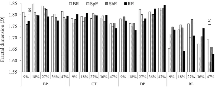
The double-log semivariogram of the loess slopes represents a linear relationship within a certain scale (Vidal et al. 2005). Therefore, the surface roughness of the loess slopes was not totally random and has a better fractal nature at certain slope gradients and ero-sion stages (Figure 6); the overall D ranged between 1.59 and 1.85. The most important factor affecting the tilled roughness of the fractal surfaces was the amplitude of the surface (Lung et al. 1999). When comparing RL surfaces of D 1.59–1.76, it was found that the overall
D was positively correlated with surface roughness.
Fractal dimension in different tillage measures. The general order of the D value of the tilled surfaces
is: RL (1.70) < CT (1.78) < DP (1.79) < BP (1.80). This suggests that the spatial autocorrelation weakened and the SH gradually strengthened due to random factors. Consequently, the spatial distribution of the surface roughness became increasingly complex.
Fractal dimension of different slope gradients. With respect to the slope steepness, the D value of the slope gradient of 27% was the highest (1.79), which indicates that the sloping surface of 27% has the high-est potential for soil erosion. The sloping surface of 47% has the lowest D value (1.76), which implies that the larger-scale variations dominate the configuration of the surface roughness and the spatial dependence is stronger than that of the other slope gradients. Thus, the sloping surface of 47% is more susceptible to erosion, reflects the critical slope gradient limit for soil and water conservation, and might be the steep-est slope gradient for effective agricultural tillage. In the Soil and Water Conservation Law of China, it is strictly prohibited to reclaim slopes steeper than 47%. Therefore, the result of this article provides a convincing reference for this clause.
Fractal dimension of different erosion stages. The D value order of the different erosion stages is the following: DSpE < DRE < DShE < DBR; small-scale variations increase. With respect to the evolution of the slope erosion, the D value decreases first and then slightly increases. This further demonstrates that the rainfall at the SpE stage initially has a relief effect on the surface roughness; it has a strengthen-ing and relief effect on the surface roughness at the ShE and REerosion stages, respectively.
CONCLUSIONS
The spatial heterogeneity (SH) of the surface rough-ness was examined in this study under
microtopo-graphic conditions. It is mainly affected by both spatial structural factors, including human cultivation activities and slope gradient, and random elements such as rainfall and soil moisture content (Vázquez
et al. 2010). Especially, the spatial configurations of the surface roughness are mainly affected by small-scale tilled measures and slope and large-small-scale rainfall and erosion processes. In general, rainfall exerts a gentle force on the surface roughness and has a certain relief effect on it. However, this effect is not notable and the size and degree of this effect are poorly understood; further studies are needed.
One legal rule of the ‘Law of the People’s Republic of China on Water and Soil Conservation’ (2010) notes that farming activities are strictly prohibited on slopes with a slope gradient > 47% (25°). Accordingly, the surface roughness on a slope of 27% (15°) has a better spatial structure and is more effective in preventing soil erosion, while the slope of 47% is more susceptible to erosion. Our results provide strong evidence for this legal rule. In general, the CT tillage measure is more feasible for the use in soil and water conservation; it prevents and controls the erosion well, regardless of the slope gradients. It can be safely popularized and applied to control the soil erosion in the sloping regions of the Chinese Loess Plateau.
[image:7.595.118.462.95.238.2]In this study, only a single rainfall intensity (2.0 mm per min) was considered. However, the surface rough-ness varies depending on different rainfall intensities, the theoretical mean sampling distance has a significant autocorrelation (3.14 m), and the maximum autocor-relation sampling distance is 12.0 m. Therefore, further research on the SH of the surface roughness and verifi-cation for a wider scale or different rainfall intensities are required. In addition, because the results might be affected by the edge effects of erosion troughs, the reliability of the results remains to be verified. Figure 6. Fractal dimension of loess tilled slopes during soil erosion process
BP – backhoe ploughing; CT – contour tillage; DP – digging ploughing; RL – rake levelling; BR – before rainfall; SpE – splash erosion; ShE – sheet erosion; RE – rill erosion;
1.85
1.59
1.65 1.70 1.75 1.80
1.85 BR SpE ShE RE
tal
di
m
en
sion-D
1.55 1.60
9% 18% 27% 36% 47% 9% 18% 27% 36% 47% 9% 18% 27% 36% 47% 9% 18% 27% 36% 47%
BP CT DP RL
Fr
ac
t
Frac
tal dimension (
D
Soil & Water Res., 13, 2018 (2): 90–97 Original Paper
https://doi.org/10.17221/130/2017-SWR
All tillage sloping surfaces of the erosion stages show a strong spatial autocorrelation and relatively stable spatial structure. The SH is a function of the scale and fractal dimension. The spatial variability of BP, CT, DP, and RL strengthens on larger scales and weakens on small scales. The surface roughness of all slopes has certain anisotropy in diverse directions on the micro-topographic scale.
Most importantly, a semivariogram-based methodo-logical framework was established in this study, which integrates the semivariogram function and anisotropy ratio with the fractal analysis featuring the SH of small-scale areas such as the surface roughness of tilled slopes. The results obtained in this study indicate that this framework is concise, applicable, and effective.
Acknowledgements. This work was financially
suppor-ted by the National Natural Science Foundation of China (41271288, 41371273), and the Fundamental Research Funds of Northwest A&F University (2452015176). The authors would like to thank all anonymous reviewers for their valuable comments which definitely improved this work.
References
Andrés P., Mathieu J., Charles L.B. (2015): How do slope and surface roughness affect plot-scale overland flow connectivity? Journal of Hydrology, 528: 192–205. Crawford C.A.G., Hergert G.W. (1997): Incorporating spatial
trends and anisotropy in geostatistical mapping of soil prop-erties. Soil Science Society of America Journal, 61: 298–309. Flagg C.B., Neff J.C., Reynolds R.L., Belnap J. (2014): Spatial
and temporal patterns of dust emissions (2004–2012) in semi-arid landscapes, southeastern Utah, USA. Aeolian Research, 15: 31–43.
Govers G., Takken I., Helming K. (2000): Soil roughness and overland flow. Agronomie, 20: 131–146.
Guedes L.P.C., Uribe-Opazo M.A., Junior P.J.R. (2013): Influence of incorporating geometric anisotropy on the construction of thematic maps of simulated data and chemical attributes of soil. Chilean Journal of Agricultural Research, 73: 414–423.
Jiang H.L., Liu G.S., Wang X.Z., Song W.F., Zhang R.N., Zhang C.H. (2010): Spatial variability of soil properties in a long-term tobacco plantation in central China. Soil Science, 175: 137–144.
Li H., Reynolds J.F. (1995): On definition and quantification of heterogeneity. Oikos, 73: 280–284.
Lung C.W., Jiang J., Tian E.K., Zhang C.H. (1999): Relation between fractal dimension and roughness index for fractal surfaces. Physical Review E Statistical Physics Plasmas Fluids & Related Interdisciplinary Topics, 60: 5121–5124. Lü Y.Z., Li B.G., Cui Y. (2006): Micro-scale spatial variance
of soil nutrients under different plant communities. Sci-entia Agricultura Sinica, 39: 1581–1588.
Moreno R.G., Burykin T., Diaz Alvarez M.C., Crawford J.W. (2012): Effect of management practices on soil mi-crostructure and surface microrelief. Applied and Envi-ronmental Soil Science, 2012: 1–9.
Pandey V., Pandey P.K. (2010): Spatial and temporal vari-ability of soil moisture. International Journal of Geo-sciences, 1: 87–98.
Peñuela A., Javaux M., Bielders C.L. (2015): How do slope and surface roughness affect plot-scale overland flow connectivity? Journal of Hydrology, 528: 192–205. Römkens M.J.M., Wang J.Y. (1984): The effect of tillage
on surface roughness. American Society of Agricultural Engineers, 84: 2026–2042.
Shen H.O., Zheng F.L., Wen L.L., Han Y., Hu W. (2016): Impacts of rainfall intensity and slope gradient on rill erosion processes at loessial hillslope. Soil & Tillage Research, 155: 429–436.
Vázquez E.V., Miranda J.G.V., Paz-Ferreiro J. (2010): A mul-tifractal approach to characterize cumulative rainfall and tillage effects on soil surface micro-topography and to predict depression storage. Biogeosciences, 7: 2099–2141. Vidal V.E., Vivas M.J.G., Paz G.A. (2005): Characterizing ani-sotropy and heterogeneity of soil surface microtopography using fractal models. Ecological Modelling, 182: 337–353. Webster R. (1985): Quantitative spatial analysis of soil in
field. Advances in Soil Science, 3: 1–70.
Wei J., Zhou J., Tian J.L., He X.B., Tang K.L. (2006): Decou-pling soil erosion and human activities on the Chinese Loess Plateau in the 20th century. Catena, 68: 10–15. WRB (2014): World Reference Base for Soil Resources,
International Soil Classification System for Naming Soils and Creating Legends For Soil Maps. 2014. World Soil Resources Reports No. 106. FAO, Rome.
Zhang Q.F., Zhao L.S., Wang J., Wu F.Q. (2014): Spati-otemporal variability and simulation of tillaged loess microtopography in water erosion. Journal of Soil and Water Conservation, 69: 343–351.
Zhang Q.F., Wang J., Zhao L.S., Wu F.Q., Zhang Z.Y., Torbert A.H. (2015): Spatial heterogeneity of surface roughness during different erosive stages of tilled loess slopes un-der a rainfall intensity of 1.5 mm∙min−1. Soil & Tillage Research, 153: 95–103.
Zhao L.S., Liang X.L., Wu F.Q. (2014): Soil surface rough-ness change and its effect on runoff and erosion on the loess plateau of china. Journal of Arid Land, 6: 400–409. Zheng F.L., Zhao J. (2004): A brief introduction on the
rainfall simulation laboratory and equipment. Research of Soil and Water Conservation, 11: 177–178. (in Chinese) Zhou Z.C., Shangguan Z.P. (2007): The effects of ryegrass
roots and shoots on loess erosion under simulated rain-fall. Catena 70: 350–355.