Department of Economics University of Southampton Southampton SO17 1BJ UK
Discussion Papers in
Economics and Econometrics
2000
THE EXACT POWER ENVELOPE OF
TESTS FOR A UNIT ROOT
Jan M. Podivinsky
¤Department of Economics
University of Southampton
Southampton SO17 1BJ
United Kingdom
Maxwell L. King
Department of Econometrics
and Business Statistics
Monash University
Clayton, Vic. 3168
Australia
Key Words and Phrases: power envelope; unit root tests.
JEL Classi…cation: C12; C22.
Abstract
We show how to obtain the exact power envelope of tests for a unit root against trend-stationary alternatives, under normality. This is in contrast to the asymptotic power envelope derived by Elliott, Rothenberg and Stock (1996), and is used to indicate the lack of power of unit root tests in …xed sample sizes.
1. INTRODUCTION
The issue of testing for a unit root in economic time series has generated a
con-siderable literature, both theoretical and empirical. Stock (1994) provides a good
up-to-date reference to this large and detailed literature. Here we address one
¤A much earlier version of some of these results was produced while the …rst author visited
particular feature of testing for a unit root, namely the exact power properties
of a common class of tests of a unit root against trend-stationary alternatives.
While this issue of exact power has received some attention in the recent
liter-ature (e.g. Bhargava (1986, 1996), Hwang and Schmidt (1993)), much of the
remaining analysis has been asymptotic in nature.
We show how to obtain the exact power envelope of tests for a unit root against
trend-stationary alternatives, under normality. This exact power envelope traces
out the maximum possible power of any such test, in a sense to be made precise
later. Evaluating the exact power envelope for this testing problem is both feasible
(making use of Dufour and King’s (1991) related analysis) and informative.
The next section outlines the precise testing problem under consideration.
Section 3 discusses the derivation and interpretation of the exact power envelope
for tests of a unit root against trend-stationary alternatives. The exact power
envelope is based upon the notion of point optimal tests introduced to
econo-metrics by King (1987a), following a related statistical literature on hypothesis
testing (e.g. Lehmann (1959), Kadilaya (1970); see also Pere (1997)). This exact
power envelope is in contrast to the asymptotic power envelope derived by Elliott,
Rothenberg and Stock (1996), and considered in Section 4. Section 5 provides a
numerical illustration of the exact power envelope, and compares it with the exact
power function for a representative unit root test. The …nal section o¤ers some
conclusions about the usefulness of the exact power envelope.
2. TESTING FOR A UNIT ROOT
The simplest possible framework for testing for a unit root takes the form of testing
the null hypothesis H0 :¯ = 1 in (e.g.) the AR(1) model with an intercept
where it is assumed (e.g.) that the errors "t s IN(0; ¾2), and y0 is an unknown
constant. However, under the alternative that¯ 6= 1this model does not allow for a trend, and so is not well-suited to testing the null hypothesis thatytis
di¤erence-stationary against the alternative hypothesis that yt is trend-stationary. Indeed,
West (1988) shows that tests in such a model are inconsistent against
trend-stationary alternatives.
Because of this, we consider an alternative framework proposed by
Bhar-gava (1986), and subsequently used by DeJong et al. (1992) and Schmidt and
Phillips (1989), that is better suited to testing di¤erence-stationarity against
trend-stationarity. For an observed time series yt we postulate
yt = ¹+®t+ut1 (2.1)
ut = ¯ut¡1+"t , "tsIN(0; ¾2)
together with some assumptions about an initial error u0. As is well known, this
can be rewritten to obtain
yt= [¹(1¡¯) +®¯] +®(1¡¯)t+¯yt¡1+"t .
Thus under the null hypothesis H0 : ¯ = 1, this simpli…es to the
di¤erence-stationary model
yt=®+yt¡1+"t ,
i.e. a random walk with drift parameter ®. However, under the (one-sided)
alternative hypothesis Ha¡:¯ <1; we obtain
yt=°+±t+¯yt¡1+"t ,
where° =¹(1¡¯)+®¯ and±=®(1¡¯). Withj¯j<1, this is a trend-stationary model. Note that the framework from which we can derive these simple
(of yt upon an intercept and a linear trend) with AR(1) errors. Also, in all that
follows, we assume that the errors "t are normally distributed.
3. DERIVATION OF THE EXACT POWER ENVELOPE
Dufour and King (1991) introduced the most powerful invariant (MPI) test of
H0 :¯ = 1, against theparticular (point) alternativeHa:¯ =¯1 (wherej¯1j<1).
In the regression error speci…cation ut=¯ut¡1+"t, we permit the AR coe¢cient
¯ to take any …nite value. Following Dufour and King (1991), we specify the
initial regression error as u0 =d0"0, where d0 6= 0is unknown, and "0 sN(0; ¾2)
independent of "t, t = 1; :::; T . We consider tests which satisfy two conditions.
Firstly, they are invariant to transformations of y = (y0; y1; y2 ;...;. yT)0 of the
form
y¤ =°0y+X° X= [¶:t]
where ¶ andt denote vectors of ones, and a linear trend respectively. Durbin and
Watson (1971) show the optimality of the Durbin-Watson statistic under such
a transformation group. Secondly, we require that the null distribution of the
test does not depend on d0, de…ned above. Dufour and King (1991) show that
this can be achieved by extending the transformation group by including in the
transformed model a dummy variable for the initial observation.
Dufour and King’s (1991) Theorem 5 provides a MPI test of the null hypothesis
H0 :¯ =¯0 against the point alternativeHa :¯ =¯1, by de…ning a point optimal
invariant (POI) test (see King (1987b) for further details) that is invariant under
the group of transformations described above, and thus has the correct size for
any d0 value. The MPI test is most powerful against the point alternative, given
the above assumptions, and is invariant by design, as described above. For our
(where j¯1j<1) takes the form of rejecting H0 for small values of
MPI(¯1; d¤0) =
v0Q0M Qv
v0v (2)
where v is a T £1 normally distributed random vector depending upon the ob-served y = (y1; y2;..., yT)0 , and Q and M are particular T £T …xed matrices, given ¯1 andd¤0. See Dufour and King (1991) for the de…nitions of v, Qand M.
Note that to apply Dufour and King’s (1991) Theorem 5, we have to specify
both a value of the point alternative ¯1 and some value (not necessarily the true
value) d¤
0 of d0. Although it would be possible to avoid the arbitrary choice of
d¤
0 by considering a larger invariance group such that the MPI test (and not just
its null distribution) does not depend on d0, Dufour and King (1991) indicate
that such tests have very inferior power properties compared with the MPI tests
considered here. In practice (as we shall see) the arbitrary choice of d¤
0 appears
to make little di¤erence to test properties.
Computationally, the principal advantage of the MPI test is that it can be
expressed as a ratio of quadratic forms in normal variables. Hence using numerical
methods (see, e.g., King (1987a) and Ansley et al. (1992)) we can calculate to
any desired accuracy both (i) theexact critical value for any desired test size; and
(ii) the exact power against any …xed alternative.
Of course, operationally the MPI test requires knowledge of, or priors upon,
the values of the …xed point alternative¯1 (<1). In most practical circumstances
this is an unrealistic assumption, and this limits that practical appeal of such MPI
tests. However, this MPI test can be used more generally to construct (empirically
or graphically) the power envelope of tests of H0 :¯ = 1, against Ha¡ :¯ < 1,
by considering a range of ¯1 values. For each point alternative within this range,
the MPI test is (by design) the most powerful test (within the invariance group)
power of any test (satisfying the given invariance property) over the region¯ <1.
It is important to note that this power envelope delineates exact powers for any
given sample size T. The power envelope indicates how de…cient (relative to this
power envelope) a particular unit root test’s power is for speci…c alternatives ¯1.
King (1990) summarises computational issues involved in evaluating the power
envelope.
4. COMPARISON WITH THE ASYMPTOTIC POWER
ENVELOPE
Elliott et al. (1996) adopt a related, but more particular, analysis. They employ a
local-to-unity asymptotic approximation to derive theasymptotic power envelope
of tests for a unit root. As with Dufour and King’s (1991) approach, and that
detailed here, they assume a normally distributed model. They argue (p. 814) that
their asymptotic power envelope analysis provides “simpler and more interpretable
results” than Dufour and King’s exact POI tests.
Their analysis covers a wider range of models than that considered here (where
attention is restricted to testing H0 : ¯ = 1 in (1)). For example, they consider
cases which allow for linear models (as in (1)) where the deterministic components
are slowly evolving. Nonetheless, a brief comparison with their analysis in the
case where the deterministic components are an intercept and a linear trend (i.e.
equation (1) above) is useful.
Their local-to-unity asymptotic approximation allows the parameter space to
c = c1 ´ T(¯1 ¡1): This test is asymptotically point optimal against the point
alternative that c = c1. The family of asymptotically point optimal tests (for
di¤erentc1 values) de…nes the asymptotic power envelope function¦(c). Each of
these tests has an asymptotic power curve tangent to the power envelope at one
point (c = c1). For the case of interest here, the asymptotic power functions of
the standard Dickey-Fuller tests are “well below” the power envelope (p. 822).
Aside from this use of the asymptotic power envelope to obtain re…ned tests, a
direct comparison with the exact power envelope is not straightforward. Because
of the local-to-unity asymptotic approximation employed, i.e. c´T(¯¡1), where
c is held constant as T ! 1, Elliott et al.’s tabulations and graphed asymptotic power envelopes are not readily interpretable without further direct evaluation.
Nonetheless, we can make some rough comparisons. For example, by inspection
from their Figure 3, which deals with the case of interest here (i.e. equation (1)),
we can see that the asymptotic power functions for the Dickey-Fuller statistics are
very close to the asymptotic power envelope for values ofcbetween0and about¡5 (or about ¡7 for the½b¿ statistic). If we take T ¼50, then this implies a range of values for¯¼1+Tc between approximately(0:9¡1), or about(0:86¡1). Thus for this local (to unity) range of ¯ values, the asymptotic power functions lie “close”
to the asymptotic power envelope. Of course, this is not directly interpretable in
terms of the exact power functions.
Elliott et al. (1996) indicate an advantage of their asymptotic power envelope
analysis over Dufour and King’s (1991) exact approach: namely that it avoids
having to make strong assumptions about the initial error u0 (and thus d¤0). The
cost of this simpli…cation, however is that their analysis is purely asymptotic.
We now consider an illustration of the alternative exact power envelope approach
5. NUMERICAL ILLUSTRATION
We consider two tests for the null hypothesisH0 :¯ = 1. One of these, based upon
the Sargan-Bhargava statistic (see Sargan and Bhargava (1983) and the extension
by Bhargava (1986)) is used as a representative test for a unit root. For example,
Edmonds et al. (1992) conclude that the Sargan-Bhargava test has comparatively
good power properties. The other test statistic is the MPI test described above,
and is used to construct the power envelope of tests for a unit root.
The Sargan-Bhargava statistic is
SB =
PT
t=2(yt¡yt¡1) 2
¡ T1¡1(yT ¡y1) 2
1 (T¡1)2
PT t=1
©
(T ¡1)yt¡(t¡1)yT ¡(T ¡t)y1¡(T ¡1)[y¡ 12(y1+yT)] ª2
This is alocally most powerful invariant test in the neighbourhood of¯ = 1of the
di¤erence stationarity null hypothesis H0 : ¯ = 1, against the trend-stationary
alternativeHa¡ :¯ <1in (1), and is invariant to the values of¹and¾2. Table I of
Bhargava (1986) gives 5% (exact) critical values for sample sizes T =f20 (5) 50 (10) 100g. Note that asSBcan be written as a quadratic form in normal variates, its size and exact power function can be evaluated by numerical methods.
The (exact) MPI test given in (2) above is used to construct the (exact) power
envelope in the following way. For a given value of d¤
0, set¯1 = 1, and use (2) to
obtain the critical value appropriate to a test of desired size. Then use this critical
value together with (2) to evaluate the rejection probability (i.e. test power) of the
MPI test against the alternative thatHa:¯ =¯1(for some¯1 satisfyingj¯1j<1).
This is, by design, a POI test against that speci…c alternative Ha : ¯ = ¯1. Of
course, given ¯1 and the appropriate critical value, the power function can be
evaluated over a range of alternative values for ¯, but only at ¯ = ¯1 will the
exact power function coincide with the power envelope. This is then repeated for
a range of¯1 values, at each stage providing another tangency point to the power
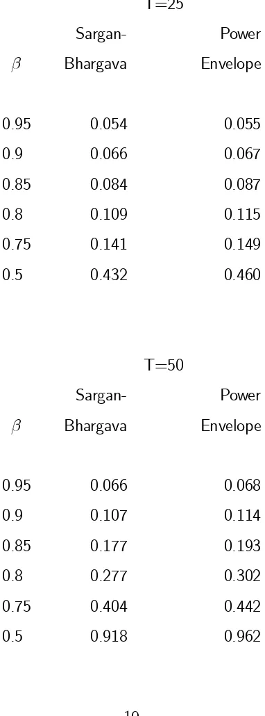
In the calculations reported in Table 1, all critical values are evaluated at exact
size 0.05. The range of values for ¯ is {1.0 0.95 0.9 0.8 0.85 0.75 0.5}, and the
powers are evaluated for two sample sizes, T = f25;50g. Note that the values reported here for the power envelope all refer to calculations assuming d¤
0 = 1.
Alternative values for d¤
0 of 0:1 or10typically made no practical di¤erence to the
calculations, and so are not reported.
The tabulations of the exact power envelope and exact power function for the
Sargan-Bhargava statistic SB indicate two key properties. First, for the sample
sizes considered here the Sargan-Bhargava test has an exact power function that
lies remarkably close to the exact power envelope, especially for ¯ close to unity.
To the extent that this test is a representative test of a unit root, with reasonably
favourable power properties compared to many competitor tests (see, e.g., Stock
(1994)), this suggests that there is little to gain (by way of increased power) by
seeking alternative tests. Note that this is not clear from Elliott et al.’s (1996)
asymptotic power envelope analysis; there the power function/power envelope
discrepancies seemed larger.
Second, this exact power envelope emphasises the following point which has
been made repeatedly in the literature but is often still ignored by practitioners.
This is that these unit root tests are not at all powerful for these sample sizes,
even against “plausible” trend-stationary alternatives not too close to the null ¯
value of unity. For example, with T = 50, the exact power envelope indicates
that no well-behaved unit root test will have power against the point alternative
¯ = 0:85 better than 0.193 ! Thus this reinforces earlier warnings (see, e.g.,
Campbell and Perron (1991) and Stock (1994)) about the possible inappropriate
TABLE 1
Exact Powers for Exact Size 0.05
T=25
Sargan- Power
¯ Bhargava Envelope
0.95 0.054 0.055
0.9 0.066 0.067
0.85 0.084 0.087
0.8 0.109 0.115
0.75 0.141 0.149
0.5 0.432 0.460
T=50
Sargan- Power
¯ Bhargava Envelope
0.95 0.066 0.068
0.9 0.107 0.114
0.85 0.177 0.193
0.8 0.277 0.302
0.75 0.404 0.442
6. CONCLUSIONS
This paper attempts to make two simple points. Firstly, obtaining information
about some exact features of unit root tests is feasible. For a standard framework
for testing for a unit root against trend-stationary alternatives, Dufour and King’s
(1991) results can be adapted to permit numerical evaluation of the exact power
envelope, without recourse to simulation methods. Secondly, this exact power
envelope can be very informative about unit root tests. This was illustrated by
a simple numerical example, with the following conclusions that reinforce earlier
simulation-based …ndings. For alternative values of ¯ near to 1, but
“represen-tative” of trend-stationary models, best possible power is awful. Also, existing
tests are “close” to attaining “best possible” power, so there is little to gain in
searching for more sophisticated (powerful) tests. If higher power is desired, what
is needed is more information, in particular more observations. Alternatively,
Hansen (1995) suggests that adding correlated covariates to the regression can
yield large power gains1.
The techniques illustrated here can be generalised, while still making use of
Dufour and King’s (1991) results. For example, their linear regression model with
AR(1) errors could be extended to “bigger” design matrices (to allow for, e.g.,
seasonal dummies, or structural breaks).
References
[1] Ansley, C.F., R. Kohn and T.S. Shively (1992), “Computingp-Values for the
Generalized Durbin-Watson and Other Invariant Test Statistics,”Journal of
Econometrics, 54(1-3), 277-300.
[2] Bhargava, A. (1986), “On the Theory of Testing for Unit Roots in Observed
Time Series,”The Review of Economic Studies, 53(3), 369-384.
[3] Bhargava, A. (1996), “Some Properties of Exact Tests for Unit Roots,”
Biometrika, 83(4), 944-949.
[4] Campbell, J.Y., and P. Perron (1991), “Pitfalls and Opportunities: What
Macroeconomists Should Know About Unit Roots,”NBER Macroeconomics
Annual, 6, 141-201.
[5] DeJong, D.N., J.C. Nankervis, N.E. Savin and C.H. Whiteman (1992),
“In-tegration Versus Trend Stationarity in Time Series,” Econometrica, 60(2),
423-433.
[6] Dickey, D.A. and W.A. Fuller (1979), “Distribution of the Estimators for
Autoregressive Time Series,”Journal of the American Statistical Association,
74, 427-431.
[7] Dufour, J.-M., and M.L. King (1991), “Optimal Invariant Tests for the
Auto-correlation Coe¢cient in Linear Regressions with Stationary or
Nonstation-ary AR(1) Errors,”Journal of Econometrics, 47(1), 115-143.
[8] Durbin, J., and G.S. Watson (1971), “Testing for Serial Correlation in Least
[9] Edmonds, G.J., R.J. O’Brien and J.M. Podivinsky (1992), “Unit Root Tests
and Mean Shifts”, Discussion Papers in Economics and Econometrics No.
9215, Department of Economics, University of Southampton.
[10] Elliott, G., T.J. Rothenberg and J.H. Stock (1996), “E¢cient Tests for an
Autoregressive Unit Root,”Econometrica, 64(4), 813-836.
[11] Fuller, W.A. (1976), Introduction to Statistical Time Series, New York:
Wi-ley.
[12] Hansen, B.E. (1995), “Rethinking the Univariate Approach to Unit Root
Testing: Using Covariates to Increase Power,”Econometric Theory, 11,
1148-1171.
[13] Hwang, J., and P. Schmidt (1993), “On the Power of Point Optimal Tests of
the Trend Stationary Hypothesis,”Economics Letters, 43, 143-147.
[14] Kadiyala, K.R. (1970), “Testing for the Independence of Regression
Distur-bances”,Econometrica, 38(1), 97-117.
[15] King, M.L. (1987a), “Testing for Autocorrelation in Linear Regression
Mod-els: A Survey,” in: M.L. King and D.E.A. Giles (eds.),Speci…cation Analysis
in the Linear Model, London: Routledge and Kegan Paul, pp. 19-73.
[16] King, M.L. (1987b), “Towards a Theory of Point Optimal Testing,”
Econo-metric Reviews, 6(2), 169-218.
[17] King, M.L. (1990), “The Power of Student’s t Test: Can a Non-Similar Test
Do Better?,”Australian Journal of Statistics, 32(1), 21-27.
[19] Pere, P. (1997),Adjusted Pro…le Likelihood Applied to Estimation and Testing
of Unit Roots, unpublished D.Phil. thesis, University of Oxford.
[20] Sargan, J.D., and A. Bhargava (1983), “Testing Residuals from Least Squares
Regression for Being Generated by the Gaussian Random Walk,”
Economet-rica, 51(1), 153-174.
[21] Schmidt, P., and P.C.B. Phillips (1992),“LM Tests for a Unit Root in the
Presence of Deterministic Trends,”Oxford Bulletin of Economics and
Statis-tics, 54(3), 257-287.
[22] Stock, J.H. (1994), “Unit Roots and Trend Breaks in Econometrics,” in
Hand-book of Econometrics, Vol. 4, ed. by R.F. Engle and D. McFadden.
Amster-dam: North-Holland, pp. 2740-2841.
[23] West, K.D. (1988), “Asymptotic Normality when Regressors have a Unit