arXiv:hep-th/0606126v2 17 Sep 2006
hep-th/0606126 AEI-2006-049 ITP-UU-06-28 SPIN-06-24
Finite-size Effects from Giant Magnons
Gleb Arutyunova,†, Sergey Frolovb,† and Marija Zamaklarb
a Institute for Theoretical Physics and Spinoza Institute
Utrecht University, 3508 TD Utrecht, The Netherlands
b Max-Planck-Institut f¨ur Gravitationsphysik, Albert-Einstein-Institut
Am M¨uhlenberg 1, D-14476 Potsdam, Germany
[email protected], [email protected], [email protected]
Abstract
In order to analyze finite-size effects for the gauge-fixed string sigma model on AdS5×S5, we construct one-soliton solutions carrying finite angular momentum J.
In the infinite J limit the solutions reduce to the recently constructed one-magnon configuration of Hofman and Maldacena. The solutions do not satisfy the level-matching condition and hence exhibit a dependence on the gauge choice, which however disappears as the size J is taken to infinity. Interestingly, the solutions do not conserve all the global charges of the psu(2,2|4) algebra of the sigma model,
implying that the symmetry algebra of the gauge-fixed string sigma model is dif-ferent from psu(2,2|4) for finite J, once one gives up the level-matching condition.
The magnon dispersion relation exhibits exponential corrections with respect to the infiniteJ solution. We also find a generalisation of our one-magnon configuration to a solution carrying two charges on the sphere. We comment on the possible impli-cations of our findings for the existence of the Bethe ansatz describing the spectrum of strings carrying finite charges.
Contents
1 Introduction and summary 2
2 String theory in a uniform gauge 8
3 Giant magnon in uniform gauge 14
3.1 Soliton solution . . . 14 3.2 Infinite J giant magnon . . . 18 3.3 FiniteJ giant magnon . . . 19
4 Global symmetry algebra 21
5 Giant magnon in the conformal gauge 23
6 Two-spin giant magnon 28
A Some explicit formulas 30
B Finite J corrections to the dispersion relation 32
1
Introduction and summary
Recent studies of string theory in AdS5 × S5 and the dual N = 4 super
Yang-Mills theory, motivated by the AdS/CFT duality conjecture [1], have led to new interesting insights into the problem of finding the spectrum of quantum strings in the AdS5 ×S5 geometry. It seems that this complicated problem can be addressed
in two stages. String states can be naturally characterized by the charges they carry under the global symmetry algebra of the AdS5×S5space-time. In the first stage one
considers states for which one of the angular momenta on the five-sphere is infinite. In this case the problem of finding and classifying the corresponding string states simplifies considerably. In the second stage, it may then be possible to bootstrap this analysis to string states with finite charges.
Perhaps the easiest way to appreciate the simplifying features of the infinite-charge limit is to consider the light-cone gauge-fixed string theory. In the light-cone gauge (for a precise definition see section 2) the gauge fixed world-sheet action depends explicitly on the light-cone momentum, which can be thought of as one of the global symmetry charges. By appropriately rescaling a world sheet-coordinate, the theory becomes defined on a cylinder of circumference proportional to the value of the light-cone momentum. At this stage, one can consider the decompactifying limit, i.e. the limit in which the radius of the cylinder goes to infinity while keeping the string tension fixed [2]-[9]. In this limit one is left with the theory on a plane which leads to significant simplifications. In particular, the notion of asymptotic states is well defined. Furthermore, since the light-cone gauge fixing manifestly breaks conformal invariance, the world-sheet theory has a massive spectrum. This theory is (believed to be) integrable at the quantum level, and hence a multi-body interaction factorises into a sequence of two-body interactions.1 Thus the problem of
solving the theory basically reduces to the problem of finding the dispersion relation for elementary excitations and the two-body S-matrix. These two quantities have not as yet been determined from the first principles of field theory. However, the insights coming from gauge theory [11]-[14] from semi-classical string quantisation [11, 15]-[20] as well as from the analysis of classical strings [21]-[26] lead to a conjecture for the form of the dispersion relation and the corresponding S-matrix [27, 28]. From the perspective of relativistic field theory, both the dispersion relation and the S-matrix have an unusual form. The dispersion relation has been conjectured to be
ǫ(p) = r
1 + λ
π2 sin 2p
2. (1.1)
The appearance of the sinp/2 in the dispersion relation is a common feature of theories on a lattice, but its origin from the world-sheet perspective remains obscure, given that the string world-sheet is continuous. Secondly, the dispersion relation is
1
not Lorentz invariant. This is basically a consequence of the gauge fixing which manifestly breaks Lorentz invariance. Yet, the dispersion relation is of relativistic form (it has a square root) signaling the possibility of having “anti-particles” in the theory, corresponding to a different choice of the sign in front of the square root.
The structure of the S-matrix was initially proposed in [28, 29, 30, 20] based on an “empirical” analysis of semiclassical string spectra. It turns out however [31], that the structure of the S-matrix is uniquely fixed by the global su(2|2)× su(2|2) ⊂ psu(2,2|4) symmetry, up to an unknown scalar function σ(p1, p2), the so-called
dressing factor. Ideally, one would hope that further physical requirements, such as unitarity, factorization and additional symmetries of the theory would uniquely fix this factor. In particular, inrelativistic integrable quantum field theories, imple-mentation of Lorentz invariance is particularly constraining. It introduces an extra equation, the crossing relation, that the S-matrix has to satisfy [32]. This equation relates the S-matrix that scatters particles with the S-matrix that scatters particles with antiparticles, and basically has a unique solution (with the minimal number of poles/zeros in the physical region).
Unfortunately, the light-cone gauge-fixed sigma model is not Lorentz invariant, and this is explicitly reflected in the Lorentz non-invariant form of the S-matrix: it depends separately on the magnon rapidities, rather than on their difference. However, it was argued in [4] that “traces” of Lorentz invariance should be present in this model and that some version of the relativistic crossing relation should hold for the S-matrix in this model. Using the Hopf-algebraic formulation of crossing in terms of an antipode, a functional equation for the dressing factor was derived in [4]. The dressing factor σ explicitly depends on the coupling √λ, and it admits a “strong coupling”, 1/√λexpansion. Currently, the first two orders in the expansion have been computed in [28, 33, 34], building upon observations of [35, 36, 37]. It was demonstrated in [8] that, up to this order, the dressing factor indeed satisfies the functional equation of [4]. It remains an important open problem to find the solution to this equation. It appears however, that the solution is not unique, and that additional physical constraints need to be imposed [38].
At largeλ the problem of deriving the dispersion relation (1.1) and the string S-matrix can be addressed in the classical string sigma model, as was recently pointed out in [9]. It was shown there that in the decompactifying limit a one-magnon ex-citation with finite world-sheet momentum p can be identified with a one-soliton solution of the classical string sigma model. The corresponding string configura-tion carries infinite energy and infinite angular momentum J, since it describes the theory on a plane. The difference of the two is, however, finite and equal to the energy of the world-sheet soliton; it is √λ/π|sin(p/2)| which is precisely the large
target space string configuration, is an open, rigidly moving string, such that the distance between the string endpoints is constant in time and is proportional to the world-sheet momentum of the magnon. In the conformal gauge supplemented by the condition t=τ this translates into nontrivial boundary conditions on the space coordinate appearing in the light-cone coordinates. A configuration with these char-acteristics was then constructed as a sigma model solution in the conformal gauge, and named the giant magnon [9].
In whatever way one solves the theory on the plane, an important problem one has to face afterwards is how to “upgrade” the findings from a plane to a cylinder. All physical string configurations are characterised by afinite value of the light-cone momentum, and as such they are excitations of a theory on a cylinder rather then on a plane. In this paper we try to systematically address the question of what kind of modification finite size effects can introduce.
In general going from a theory on a plane to a theory on a cylinder may modify the theory significantly. While on a plane it is always possible to construct a multi-particle state as a superposition of well-separated single-multi-particle excitations, this is no longer the case once we are on a cylinder. However, if the size of the cylinder L
is very large, much larger than the size of the excitation and much larger than the range of the interactions, then the leading finite-size effects could be incorporated through the following asymptotic construction. The dispersion relation for a single excitation is taken to be the same as in the infinite volume system, the energy of a multi-particle system is taken to be additive, and the structure of the wave function is unmodified. The only way in which finite-size effects modify the consideration from the plane, is via periodic boundary conditions which eigenstate wave functions have to satisfy. In the case of a spin chain, the boundary conditions on the wave function basically lead to Bethe equations. In some cases, like for example for the XXX spin chain, this asymptotic construction remains exact for any size of the finite-size system. However, for spin chains with long-range interactions, such are those which arise in higher-order perturbation gauge theory, the asymptotic construction is valid only for long spin chains. Once the range of interactions between magnons becomes of the size of the system, the asymptotic construction has to be modified, and finite-size effects (the wrapping interactions in the gauge theory language) have to be taken into account.
it in the classical theory, and construct solutions of the sigma model corresponding to a single magnon excitation for the theory on a cylinder. We find magnon solutions of the string sigma model in the conformal gauge and in a one-parameter family of light-cone gauges, labeled by a parameter a,
x+ = (1−a)t+aφ=τ , x−=φ−t , p+= (1−a)pφ−a pt= const. (1.2)
Many new features appear with respect to the case of infinite volume. The first and probably the most striking result at first glance, is that a magnon in the finite size system is a gauge dependent object: its target space picture and the disper-sion relation explicitly depend on the parametera. Furthermore, all of these various magnon configurations reduce tothe same configuration in the limit of infinite light-cone momentum, i.e in the limit where the size of the system is taken to infinity. Both of these results however should not come as a surprise. Namely, one way of “constructing” a single magnon configuration is to start with the physical, closed string state which describes the system of two magnons (with vanishing total world-sheet momentum). To isolate a one-magnon state, we need to cut this closed string, and separate the magnons from each other. In principle, cutting of the string is an unphysical process, since its obviously breaks reparametrisation invariance (it declares that different parts of the string are physically different). Hence cutting of the string may introduce gauge dependence, depending on how we decide to open the string. A natural way of opening the string is dictated by dropping the level matching condition. In the light-cone gauges (1.2) it implies that
∆x− =− Z √π
λP+
−√π
λP+
dσpixi′ 6= 0, (1.3)
whereP+ is the total light-cone momentum andxi andpi are transverse coordinates
and momenta. In other words, if level matching is not satisfied in the gauge labeled by a, the string opens in the x− direction, so that the separation of its endpoints in this direction is constant with respect to the time x+. Note however, that the
derivatives of the transverse fields xi do not vanish at the string endpoints, and
hence correspondingly the sheet momentum does not vanish there. The world-sheet momentum is however conserved, as a consequence of the periodic boundary conditions whichpi, xi satisfy. In other words, although the world-sheet momentum
“flows out” of the string on one side, it “flows in” from the other side, due to the periodic boundary conditions.
Figure 1: There are potentally two ways to take the limit from a finiteJ, two soliton configuration. One way is to have the solitons on “different sides” of the string: this leads to two one-soliton configurations, living on different lines. Another way is to have the solitons on the same “side” of the string: this leads to a nontrivial two-soliton configuration on the line. In the target space, the former configuration corresponds to a folded string with the shape of a giant magnon, which is a legitimate closed string state. In the latter case, sendingJ to infinity, does not naturally opens up the string, since solitons remain unseparated in the limit. Only if the total worldsheet momentum is nonzero, the latter becomes a complicated open string state, which is such that when the total worldsheet momenta of solitons becomes zero, one is back to the closed string.
Figure 2: At finiteJ the two-soliton configuration is complicated and never a trivial superposition of two one-magnon solutions. This is the reason why we cannot trivially build a closed string state only from two magnons. At infiniteJ
the situation is different, and there is a trivial configuration of two magnons (see the upper right-hand side picture of figure 1).
Although our one-magnon configurations are gauge dependent, the requirement that the spectrum of physical excitations is gauge independent imposes severe con-straints on the structure of the theory. It is plausible that for finite J, there is a preferred choice of the parametera simplifying the exact quantisation of the model. Our analysis indicates that it would be the temporal gauge, t =τ , pφ =J,
corre-sponding to a= 0. The suggestive reason for this is that, as we show in this paper, only for the a = 0 gauge one can identify the world-sheet momentum (2.14) with the spin-chain magnon momentum.
The second result of our analysis is that the dispersion relation for the one-magnon case receives exponential corrections with respect to the infinite J case.
E−J =
√
λ π sin
pws
2
1− 4
e2 sin 2 pws
2 e
where R is the effective length felt by the magnon with momentum pws
R = √ 2πJ
λsin pws
2
+apwscot
pws
2 .
This formula shows explicitly a nontrivial dependence on the parametera. Moreover, the dispersion relation is periodic in pws only for a= 0. This is the reason why the
a= 0 gauge seems to be preferred from a gauge theory perspective.
It is known that the one-magnon configuration is half-supersymmetric, i.e. the energy of the magnon (1.1) is determined by the BPS relation (1.1) which follows from the centrally extended su(2|2)×su(2|2) algebra [31, 9]. Still, the magnon
energy receives finite-size corrections, and this implies that the central charge in the algebra should also receive finite-size corrections.
This brings us to the third result of our analysis. Namely, by explicitly evaluating the charges of the SO(3) algebra on our one-magnon configurations, one can check that the off-diagonal charges are not preserved in time.2 As we explicitly show
(see section 4) this is a simple consequence of the fact that one dismisses the level matching condition, and of the fact that the transverse fields do not satisfy Neumann boundary conditions. If J is infinite, all charges are conserved since the open string satisfies standard boundary conditions.
The breaking of the algebra may sound worrisome. A similar phenomenon has however already appeared in the case of the asymptotic all-loop Bethe ansatz in [30], where only after imposing the momentum conservation one recovered the full psu(2,2|4) algebra.3 Also, the algebraic construction of the S-matrix in [31]
involved only the su(2|2)×su(2|2) subalgebra, rather then the full psu(2,2|4)
alge-bra. It would be very important to understand the structure of the finiteJ, off-shell algebra more explicitly.
In the last section we generalise our finite J magnon configuration to the case of two spins. In the infinite J limit this configuration reduces to the two-spin giant magnon solution of [39]. Our method to obtain this solution is however different from the one used in [39] and may be more applicable for the construction of the three-spin configuration.
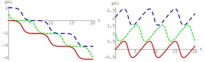
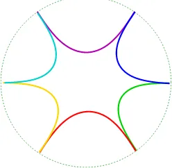
Finally, let us comment on the target space picture of the finite-size giant magnon. A simulation of the time evolution of the solution in the conformal and
a= 0 gauges can be seen at http://www.aei.mpg.de/~peekas/magnons/. Several snapshots from this movie are shown in figure 3. We see that, unlike the infinite J
magnon, the string configuration is nonrigid: propagation of the soliton from one end of the string to the other happens in a finite target space time, and leads to “wiggly” behavior of the string. The boundaries of the “stripe” in which the string wiggles depend onJ and the world-sheet momentump. There are three limits which
2
Rephrasing F. Dostoevsky, we could summarise our findings in one sentence: “If there is no God, everything is broken”.
3
Figure 3: Snapshots of the time evolution of the solution in conformal gauge.
one can take, and which link our solution to the known string configurations. These thus serve as a crosscheck of the solution. First, as J → ∞ the solution reduces to the solution of [9]. The string endpoints touch the equator and the period with which the string wiggles goes to infinity. Secondly, if we keep J finite, and send the world-sheet momentum to its maximal value p= π, the solution reduces to half of the rigid folded string of [15]. Finally, as the world-sheet momentum is sent to zero, the giant magnon “shrinks” to zero size, and reduces to a massless point particle moving on the equator with the angular momentum equal to J.
We end the introduction with a summary of the potential implications of our findings to the Bethe ansatz approach to the quantisation of strings. The crucial feature necessary for the formulation of the Bethe ansatz, is additivity of the energy for the multi-magnon excitations. This feature seems to be lost in the case of the finite J configurations. Namely, giant magnons correspond to world-sheet solitons. Typically multi-soliton configurations are not simple superpositions of one-soliton configurations, neither for finite nor for infinite spaces. In addition, in finite volumes the very definition of soliton number becomes obscure. Yet, in our case it seems that there exists a (at least heuristic) way of counting the number of solitons present in the finite J string. These should correspond to the number of (target space) spikes characterising the string configuration. However, as explained in section 4 the energy of such a multi-magnon configuration would not generically be realised as the sum of the energies of one-magnon configurations, carrying the appropriate fraction of the total charge. This seems to imply that at finite J the string spectrum would not be described by a simple Bethe ansatz of the form [28]. If the Bethe ansatz description of the string spectrum at finite J is at all possible, then it is plausible that this would require the introduction of auxiliary excitations similar to the constructions of [2, 40, 6, 41, 42].
2
String theory in a uniform gauge
We consider strings propagating on a target manifold possessing (at least) two abelian isometries realized by shifts of the time coordinate of the manifold denoted by t, and a space coordinate denoted by φ. If the variable φ is an angle then the range of φ is from 0 to 2π.
To impose a uniform gauge we also assume that the string sigma-model action is invariant under shifts of t and φ, with all the other bosonic and fermionic fields being invariant under the shifts. This means that the string action does not have an explicit dependence ont and φand depends only on the derivatives of the fields. An example of such a string action is provided by the Green-Schwarz superstring in AdS5×S5 where the metric can be written in the form
ds2 =Gttdt2 + Gφφdφ2 + Gijdxidxj.
Here t is the global time coordinate of AdS5, φ is an angle of S5, and xi are the
remaining 8 coordinates of AdS5×S5. Strictly speaking, the original Green-Schwarz
action presented in [49] contains fermions which are charged under the U(1) trans-formations generated by the shifts oft andφ. However, it is possible to redefine the fermions and make them neutral, see [47, 50] for details.
To simplify the notations we consider explicitly only the bosonic part of a string sigma model action, and assume that the B-field vanishes. A most general fermionic Green-Schwarz action can be analyzed in the same fashion, and leads to the same conclusions. The corresponding part of the string action can be written in the following form
S =− √
λ
4π
Z r
−r
dσdτ γαβ∂αXM∂βXNGM N. (2.1)
Here √λ
2π is the effective string tension, which for strings in AdS5 ×S
5 is related
to the radius of S5 as √λ = R2/α′. Coordinates σ and τ parametrize the string
world-sheet. For later convenience we assume the range of σ to be −r ≤ σ ≤ r, where r is an arbitrary constant. The standard choice for a closed string is r =π. Next,γαβ ≡√−h hαβ is a Weyl-invariant combination of the world-sheet metrichαβ
which in the conformal gauge is equal toγαβ = diag(−1,1). Finally, XM ={t, φ, xi}
are string coordinates and GM N is the target-space metric which is independent of
t and φ.
The simplest way to impose a uniform gauge is to introduce momenta canonically-conjugate to the coordinatesXM
pM =
2π
√
λ δS
δX˙M =−γ
0β∂
βXNGM N, X˙M ≡∂0XM, (2.2)
and rewrite the string action (2.1) in the first-order form
S =
√
λ
2π
Z r
−r
dσdτ
pMX˙M +
γ01
γ00C1+
1 2γ00C2
The reparametrisation invariance of the string action leads to the two Virasoro constraints
C1 =pMX′M, C2 =GM NpMpN +X′MX′NGM N, X′M ≡∂1XM,
which are to be solved after imposing a gauge condition.
The invariance of the string action under the shifts leads to the existence of two conserved charges
E =−
√
λ
2π
Z r
−r
dσ pt , J = √
λ
2π
Z r
−r
dσ pφ . (2.4)
It is clear that the charge E is the target space-time energy andJ is the total U(1) charge of the string.
To impose a uniform gauge we introduce the “light-cone” coordinates and mo-menta:
x− =φ − t , x+ = (1−a)t + a φ , p− =pφ + pt , p+ = (1−a)pφ − a pt ,
t=x+ − a x− , φ=x+ + (1−a)x− , pt= (1−a)p−−p+ , pφ=p+ + a p− .
Here, a is an arbitrary number which parametrizes the most general uniform gauge up to some trivial rescaling of the light-cone coordinates such that the light-cone momentum p− is equal topφ + pt. This choice of gauge is natural in the AdS/CFT
context because, as we will see in a moment, in a uniform gauge the world-sheet Hamiltonian is equal to E − J. Taking into account (2.4), we get the following expressions for the light-cone charges
P− =
√
λ
2π
Z r
−r
dσ p− = J − E , P+ =
√
λ
2π
Z r
−r
dσ p+ = (1−a)J + a E .
In terms of the light-cone coordinates the action (2.3) takes the form
S =
√
λ
2π
Z r
−r
dσdτ
p−x˙++p+x˙−+pix˙i+
γ01
γ00C1+
1 2γ00C2
, (2.5)
where
C1 = p+x′− + p−x′+ + pix′i, (2.6)
and the second Virasoro constraint is a quadratic polynomial inp−. We then fix the uniform light-cone gauge by imposing the conditions
x+ = τ + amσ , p+ = 1 . (2.7)
The integer number mis the winding number which appears because the coordinate
φ is an angle variable with the range 0 ≤ φ ≤ 2π. The consistency of this gauge choice forces us to choose the constant r to be
r= √π
To find the gauge-fixed action, we first solve the Virasoro constraint C1 for x′−
C1 = x′− + amp− + pix′i = 0 =⇒ x′− = −amp− − pix′i, (2.9)
substitute the solution to C2 and solve the resulting quadratic equation for p−.
Substituting all these solutions into the string action (2.5), we end up with the gauge-fixed action
S =
√
λ
2π
Z r
−r
dσdτ pix˙i − H
, (2.10)
where
H = −p−(xi, x′i) (2.11)
is the density of the world-sheet Hamiltonian which depends only on the physical (transverse) fields xi. It is worth noting that H has no dependence on λ, and the
dependence of the gauge-fixed action on P+ comes only through the integration
limits ±r.
The world-sheet Hamiltonian in this gauge is related to the target space-time energy E and the U(1) charge J as follows
H =
√
λ
2π
Z r
−r
dσH=E−J . (2.12)
In the AdS/CFT correspondence the space-time energy E of a string state is iden-tified with the conformal dimension ∆ of the dual CFT operator: E ≡ ∆. Since the Hamiltonian H is a function of P+ = (1−a)J +aE, for generic values of a
the relation (2.12) gives us a nontrivial equation on the energy E. Computing the spectrum of H and solving the equation (2.12) would allow us to find conformal dimensions of dual CFT operators.
There are three natural choices of the parameter a. Ifa= 0 we get the temporal gauge t=τ , p+ =J. For strings moving in the R×S
5 subspace of AdS
5 ×S5 this
gauge choice is related to the conformal gauge supplemented by the conditiont =τ
we use in section 5 to find the finite E one-magnon configuration. It was shown in [25] that this gauge was (implicitly) used in [19] to compute 1/J corrections in the near BMN limit [11], and that the gauge-fixed Hamiltonian describes an integrable model. It is clear that the consideration of [25] can be straightforwardly generalized to any a and therefore, for fixed λ , P+, m, the gauge-fixed Hamiltonians define
a one-parameter family of integrable models. If a = 1
2, we obtain the uniform
light-cone gauge x+ = 12(t+φ) = τ , P+ = 12(E +J) introduced and used in [48]
to analyze the su(1|1) subsector (see also [51]). The light-cone gauge appears to
ansatz [28] in a simpler form [20]. Finally, one can also set a = 1. In this case, the uniform gauge reduces to x+ = φ = τ , P+ = E, where the angle variable φ
identified with the world-sheet timeτ, and the energyE distributed uniformly along the string. String theory in AdS5×S5 has not been analyzed in this gauge yet.
Since we consider closed strings, the transverse fields xi are periodic: xi(r) =
xi(−r). Therefore, the gauge-fixed action defines a two-dimensional model on a
cylinder of circumference 2r = √2π
λP+. In addition, the physical states should also
satisfy the level-matching condition
∆x− = Z r
−r
dσx′− = √2π
λamH −
Z r
−r
dσpix′i = 2πm . (2.13)
The gauge-fixed action is obviously invariant under the shifts of the world-sheet coordinateσ. This leads to the existence of the conserved charge
pws =−
Z r
−r
dσpix′i, (2.14)
which is just the total world-sheet momentum of the string. In what follows we will be interested in the zero-winding number case, m = 0. Then the level-matching condition just says that the total world-sheet momentum vanishes for physical con-figurations
∆x− =pws = 0, m= 0. (2.15)
The gauge-fixed action can be used to analyze string theory in various limits. One well-known limit is the BMN limit [11] in which one takes the λ → ∞ and
P+ → ∞ while keeping ˜λ = λ/P+2 fixed. In this case it is useful to rescale σ so
that the range of σ would be from −π to π. The gauge-fixed action admits a well-defined expansion in powers of 1/P+, with the leading part being just a quadratic
action for 8 massive bosons (and 8 fermions). The action can be easily quantized perturbatively, and used to find 1/P+ corrections [19, 20].
Another interesting limit is the decompactifying limit whereP+→ ∞withλkept
fixed. In this limit the circumference 2rgoes to infinity and we get a two-dimensional model defined on a plane. Since the gauge-fixed theory is defined on a plane the asymptotic states and S-matrix are well-defined. This limit has been studied in [3]-[9]. An important observation recently made in [9] is that in the limit one can give up the level-matching condition and consider configurations with arbitrary world-sheet momenta. Then, a one-soliton solution of the gauge-fixed string sigma model should be identified with a one-magnon state in the spin chain description of the gauge/string theory [12, 27, 28, 30], and the world-sheet momentum is just equal to the momentum of the magnon
The corresponding one-soliton solutions were named giant magnons in [9] because generically their size is of order of the radius of S5. Since for a giant magnon ∆x
−
is not an integer multiple of 2π, such a soliton configuration does not describe a closed string. It was shown in [9] that the classical energy of a string giant magnon is related to the momentum pws by the formula
Estring=
√
λ π
sinpws 2
, (2.17)
which is the strong coupling, (i.e.λ→ ∞) limit of the spin chain dispersion relation [27]
Espin chain =
r 1 + λ
π2 sin 2p
2, p≡pmagnon. (2.18)
This is an interesting result because the appearance of trigonometric functions is usually associated with a lattice structure, while here the dispersion relation was derived in a continuous model. Moreover, the semi-classical S-matrix was also com-puted in [9], and shown to coincide with the semi-classical approximation of the quantum string Bethe ansatz S-matrix of [28].
In this paper we want to stress that it is natural to give up the level-matching condition not only in the decompactifying limit but also for finite P+. The reason
is that to quantize string theory in a uniform gauge one has to consider all states with periodic xi, and impose the level-matching condition only at the end to single
out the physical subspace. In a uniform gauge one still has a well-defined model on a cylinder, however, if a string does not satisfy the level-matching condition then its target space-time image is an open string with end-points of the string moving in unison so that ∆x− remains constant. Another subtlety is that it is the level-matching condition that makes gauge-fixed string sigma models equivalent for different choices of a uniform gauge, that is for different values of a. String configurations which do not satisfy the level-matching condition may depend on a. This gauge-dependence makes the problem of quantizing string theory in a uniform gauge very subtle. On the other hand the requirement that physical states are gauge independent should impose severe constraints on the structure of the theory. It may also happen that for finite J there is a preferred choice of the parameter a
simplifying the exact quantization of the model. In fact we will see that for finite
In the strong coupling limitλ→ ∞one should be able to use the classical string theory to find a corresponding one-soliton solution4 and determine the finite P
+
corrections to the dispersion relation (2.17). This is the problem we are going to address in the next sections.
3
Giant magnon in uniform gauge
As was discussed in [9], a giant magnon is a string moving on a two-dimensional sphere. This is a consistent reduction of classical string theory on AdS5×S5. Our
starting point is the bosonic action (2.1) for strings in R×S
2
S =−
√
λ
4π
Z r
−r
dσdτ γαβ(−∂αt∂βt+∂αXi∂βXi) , (3.1)
where XiXi = 1. We find convenient to use the following parametrization of S2
X1+iX2 =
√
1−z2eiφ, X
3 =z , −1≤z ≤1. (3.2)
The coordinate z is related to the standard angleθ asz = cosθ. The valuesz =±1 correspond to the north and south poles of the sphere, and at z = 0 the angle φ
parametrizes the equator. In terms of the coordinatesφand zthe metric ofS2 takes
the form
ds2S2 =
dz2
1−z2 + (1−z
2)dφ2. (3.3)
3.1
Soliton solution
Introducing the light-cone coordinates (2.5), imposing the uniform gauge (2.7) (with
m = 0), and following the steps described in the previous section, we derive the gauge-fixed string action
S =
√
λ
2π
Z r
−r
dσdτ (pzz˙ − H), (3.4)
where the density of the gauge-fixed Hamiltonian is a function of the coordinate
z and its canonically conjugate momentum pz. Recall also that r = √πλP+ =
π
√
λ ((1−a)J+aE). Explicit expressions for the Hamiltonian and other quantities
computed in this section can be found in Appendix A where we also present their forms for the three simplest cases a= 0,1/2,1.
4Strictly speaking, since for finite P
+ the theory is defined on a cylinder, the corresponding
To find a one-soliton solution of the gauge-fixed string theory it is convenient to go to the Lagrangian description by eliminating the momentum pz. Solving
the equation of motion for pz that follows from the action (3.4), we determine the
momentum as a function of ˙z and z. Then substituting the solution into (3.4), we obtain the action in the Lagrangian form: S =S(z, z′,z˙). The explicit form of the
action is given in Appendix A, and it is of the Nambu-Goto form. We will see in a moment that this leads to the existence of finite-energy singular solitons.
To find a one-soliton solution we make the most general ansatz describing a wave propagating along the string
z =z(σ−vτ), (3.5)
where v is the velocity of the soliton. Substituting the ansatz into the action (A.3), we derive the Lagrangian,Lred=Lred(z, z′), of a reduced model which defines a
one-particle system if we regardσas a time variable. Theσ-evolution of this system can be easily determined by introducing the “momentum” conjugated to z with respect to “time” σ
πz =
∂Lred
∂z′ ,
and computing the reduced Hamiltonian
Hred=πzz′−Lred.
The reduced Hamiltonian is a conserved quantity with respect to “times” σ, and we set it to some constant
Hred=
ω−1 1−a+a ω.
Here we have chosen to parametrise the constantHredin this way in order to simplify
the comparison with the conformal gauge solution in section 5.
Solving this equation with respect to z′, we get the following basic equation
z′2 =
1−z2
(1−a) (b2 −z2)
2
z2−z2
min
z2
max−z2
, (3.6)
where the parameters zmin, zmax and b are related to a,v and ω as follows
zmin2 = 1− 1
ω2 , z 2
max = 1−v2, b2 = 1 +
a
(1−a)ω. (3.7)
A one-soliton solution we are looking for corresponds to a periodic solution of the equation (3.6), the period being equal to 2r = √2π
λP+. The parameter zmin is
-1 -0.5 0.5 1 0.3
0.4 0.5 0.6 0.7 0.8 0.9 1 z
σ
-1 -0.5 0.5 1
-3 -2 -1 1 2 3
x−
[image:17.612.115.484.65.193.2]σ
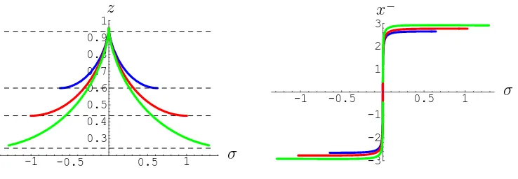
Figure 4: Profile of a= 0 one-magnon soliton: Left,z(σ) plotted for configura-tions with the same zmax= 0.99 andzmin={0.6,0.19,0.06}, green, red and blue
respectively. Right, profilex−(σ) for the same values of zmin, zmax.
It is not difficult to see that such a solution exists if the following inequalities hold
0≤a≤1, 0≤zmin2 ≤zmax2 ≤b2. (3.8)
It follows from these inequalities that the range of a, ω and v is
0≤a≤1, 1≤ω <∞, 0≤ |v| ≤ 1
ω. (3.9)
Then, assuming for definiteness that z ≥ 0, the corresponding solution of the equation (3.6) lies between zmin and zmax, and for givena andv the parameterzmin
is found from the equation
r= Z r
0
dσ = Z zmax
zmin
dz
|z′|. (3.10)
This integral can be easily computed in terms of elliptic functions by using formulas from Appendix B.
One can easily see from equation (3.6) that in the range of parameters (3.8) the shape of the soliton is similar for any values of a, v and ω. The allowed values of z
are zmin ≤ z ≤ zmax, and z′ vanishes at z =zmin, and goes to infinity at z =zmax.
So, if we assume that atτ = 0 the solution is such that z′ = 0 atσ =−r andσ =r,
then z =zmax atσ = 0, and the soliton profile is shown in Fig.(4).
The corresponding solution is, as we see, not smooth at z = zmax. The energy
of this soliton is however finite. To compute the energy, we need to evaluate H/|z′|
on the solution:
H |z′| =
z2 −(ω−1)1
ω +
(1−a)v2
1−a+aω
− v2
1−z2
a(ω−1)
ω(1−a+aω)
p (z2
max−z2)(z2−zmin2 )
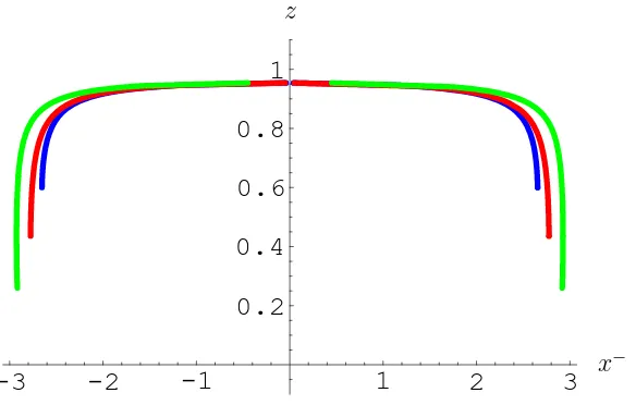
-3
-2
-1
1
2
3
0.2
0.4
0.6
0.8
1
z
[image:18.612.162.454.69.255.2]x−
Figure 5: Target space shape of magnon at fixed light-cone time x+, depicted for three magnons moving in the stripe zmax = 0.99, zmin = {0.6,0.19,0.06},
green, red and blue respectively.
Then the energy of the soliton is given by the following integral
E−J =
√
λ
2π
Z r
−r
dσH=
√
λ π
Z zmax
zmin
dz H
|z′|, (3.11)
and it is clear from this expression that the energy is finite.
Finally, we also need to compute the world-sheet momentum (2.14)
pws =−
Z r
−r
dσpzz′ = 2 Z zmax
zmin
dz|pz|, (3.12)
where we have assumed that v > 0, and took into account that then for the soli-ton we consider the product −pzz′ is positive. The following explicit formula for
the momentum pz canonically conjugate to z can be easily found by using
equa-tion.(A.2),(3.5) and (3.6)
pz =
vω
1−a+aω
1 1−z2
p
z2−z2
min p
z2
max−z2
. (3.13)
Let us also mention that in the case of a one-soliton solution the world-sheet mo-mentum (3.12) is just equal to the canonical momo-mentum carried by the center of mass of the soliton. To see that we just need to plug the ansatz (3.5) into the string action (3.4), and integrate over σ. Then we obtain the following action for a point particle
S =
√
λ
2π
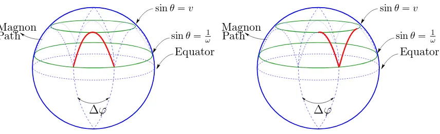
Z
Magnon Path
Equator
sinθ= 1
ω sinθ=v
∆ϕ
Magnon Path
Equator
sinθ= 1
ω sinθ=v
[image:19.612.104.532.61.192.2]∆ϕ
Figure 6: Plot of the time evolution of the finite J magnon on the sphere. Left picture depicts moment t = 0, while the right t = T /4 , where T is period:
T = 2r/v. We see that string develops a spike during the time evolution.
that shows explicitly that pws is the soliton momentum.
It is also useful to understand the target-space shape of the soliton, that is to find the dependence ofz on the target-space coordinatex−. To this end we compute the derivative dz/dx−
dz dx− = z′ x′ − = 1 pz
= 1−a+aω
vω (1−z
2)
p
z2
max−z2 p
z2 −z2
min
. (3.14)
We see that in the target space, the soliton configuration is in fact smooth at z =
zmax and singular at z = zmin. Then the configuration is not static, see Fig.6 and
the simulations at http://www.aei.mpg.de/~peekas/magnons/.
3.2
Infinite
J
giant magnon
To recover the uniform gauge equivalent of the giant magnon solution of [9] we need to send r to infinity. It is easy to see that this limit corresponds to setting the parameter zmin to 0 or equivalently ω to 1. In the limit ω → 1 the basic equation
(3.6) simplifies
z′2 =
z(1−z2)
(1−(1−a)z2)
2
1
1−v2−z2 , (3.15)
and can be easily integrated. The range of σ is now from −∞ to ∞, and both z′
and z vanish atσ =±∞. Even though the solutionz(σ−vτ) depends ona, for all values ofa from the interval [0,1] the energy (3.11) and the world-sheet momentum (3.12) depend only on v
E−J =
√
λ π
Z zmax
zmin
dz H
|z′| =
√
λ π
Z √1−v2
0
dz√ z
1−v2−z2 =
√
λ π
√
1−v2,
pws = 2
Z zmax
zmin
dz|pz|= 2
Z √1−v2
0
dz vz
Expressingvin terms ofpws, we get the dispersion relation (2.17). This demonstrates
explicitly that in the infinite J limit one can give up the level-matching condition and still have independence of the gauge choice. We will see in the next subsection that it is not the case for finite J.
3.3
Finite
J
giant magnon
To find the dispersion relation for finite J we need to express the soliton energy
E −J in terms of J and the world-sheet momentum pws. It is obvious that there
is no simple analytic expression for the dispersion relation. It is possible however to analyze dispersion relation for large values of the charge J. The details of this complicated analysis are given in Appendix B. All corrections turn out to be only exponential in this limit. The leading and subleading exponential corrections to
E−J computed in the appendix are
E−J =
√
λ π sin
pws
2 h
1− 4
e2 sin 2 pws
2 e
−R− (3.16)
− 4
e4 sin 2 pws
2
R2(1 + cosp
ws) + 2R(2 + 3 cospws+apwssinpws) +
+ 7 + 6 cospws+ 6apwssinpws+a2p2ws(1−cospws)
e−2R+· · ·i.
Here we have introduced the effective length felt by the magnon with momentum
pws
R = √ 2πJ
λsin pws
2
+apwscot
pws
2 . (3.17)
Formula (3.16) has several interesting features. First of all it shows that the expo-nential correction is basically determined by the ratio J/(E −J) because for large values of J, R ∼2J/(E−J). Then, for generic values ofa the dispersion relation is not periodic in pws. The periodicity in pws is restored only for a = 0. This
indi-cates that for finiteJ one can identify the world-sheet momentum with a spin-chain magnon momentum only for a= 0.
Formula (3.16) also shows a nontrivial dependence on the parametera. Only the coefficients of the leading terms, e−RandR2e−2R, are independent ofa. The
depen-dence must, however, disappear in the casev = 0 which corresponds to the finite-J
generalization of the “half-GKP” solution [15] describing an open string satisfying the Neumann boundary conditions and rotating on S2 with spin J. Computing the
world-sheet momentum in the limit v →0, we find
pws →
π
1−a+aω . (3.18)
Thus, pws →π only in the case a= 0 or in the case ω = 1 that corresponds to the
changes from −π to π (we consider a zero-winding case), we see that pws can be
naturally identified with pmagnon only for a= 0.5 Now taking into account that ω is
a function of a and J, we find that in the limit v → 0 the world-sheet momentum has the following expansion
pws =π−
8πa e2 e
−J + 32πa(−1 + 2a+J) e4 e
−2J +· · · , (3.19)
Substituting this formula into (3.16), we obtain the following formula for the expo-nential correction to the energy of the “half-GKP” solution
E−J =
√
λ π
h 1− 4
e2e−J −
4
e4(1−2J)e−
2J +· · ·i, (3.20)
whereJ = 2√πJ
λ. This expression has noa-dependence as it should be. The fact that
there is no a-dependence in this case also follows from exact equations (B.7) and (B.8) in Appendix B without performing any expansion.
Let us also mention that the GKP folded string rotating on S2 with spin J [15]
can be thought of as being composed from two giant magnons with spin J/2 and
pws =π. The energy of the folded string is still equal to the sum of energies of the
magnons even at finiteJ. In fact, in thea= 0 gauge ifpws = 2πmN we can also build
a closed string configuration with the winding number m carrying the charge J by gluingN finiteJ/N solitons, see section 5 for a discussion of this configuration, and Fig.(10), (11) and (12). The resulting configuration was analyzed in [53], and is an S2-analogue of the AdS
3 spiky strings studied in [52], and the energy of this closed
string is again equal to the sum of energies of the N magnons.
In general, however, we expect the simple addition formula for the energy of a composite closed string to be correct only at infinite J where all the exponential corrections in (3.16) vanish. If so then at finite J the string spectrum would not be described by a simple Bethe ansatz of the form [28]. If a Bethe ansatz description of the string spectrum is possible at all then it would have auxiliary excitations and a more complicated dispersion relation with the usual one (2.18) arising only at infinite
J similar to what happens in the Hubbard model description of the BDS spin chain [40]. It is worth noting that in the Hubbard model the exponential corrections to the dispersion relation are also governed by the same effective lengthR(3.17) (with
a= 0). However, one can check, that these corrections appear only in the subleading orders in 1/√λ. The strong coupling dispersion relation (2.17) is not modified in the Hubbard model, unlike what is observed here. Similarly, the quantum, finite size corrections computed in [3], seems to predict that the same exponential term governs finite size corrections at the quantum level.
5In principle one could rescale the momentum by a factor depending onJ and a so that the
It is also worth stressing that at largeλ a realistic quantum string Bethe ansatz should lead to the same exponential correction for the dispersion relation, and that our result should serve as a nontrivial check of any proposal for such an ansatz. Note also that not only exponential terms, but also highly non-trivial coefficients multiplying series in R need to be reproduced.
4
Global symmetry algebra
In this section we discuss the implications of giving up the level-matching condition for the global symmetry algebra of a string model.
Recall that the theory we consider is obtained by reduction of the string sigma-model on AdS5 ×S5 to a smaller space R ×S
2. This space still has a non-trivial
isometry group which is R×SO(3), where R corresponds to the shifts of the global AdS time t and SO(3) is the isometry group of the two-sphere. It is known that giving up the level-matching condition leads to dramatic consequences for the global symmetry algebra, namely, it gets reduced, because some of the global charges fail to satisfy the conservation law.
This phenomenon is of course general and it also occurs for closed strings prop-agating in flat space. Indeed, in the light-cone gauge the dynamical generators of the Lorentz algebra are given by
Ji−= Z 2π
0
dσ(XiX˙−−X−X˙i).
Using the flat string equations of motion XM = 0 for M = i,− the (total) time
derivative of these generators can be reduced to the total derivative term
˙
Ji− = Z 2π
0
dσ(XiX¨−−X¨iX−) =−Xi′(0)X−(2π)−X−(0),
where we have used the fact that the transversal fields Xi,(Xi)′ are periodic. If
the level-matching condition is not satisfied, i.e. ∆X− = X−(2π) −X−(0) 6= 0
the dynamical generators of the Lorentz algebra are broken. Only for special con-figurations, for which the transversal coordinates obey the open string condition
Xi′(0) = 0 = Xi′(2π) the dynamical generators in question are still conserved. This
picture has a clear physical meaning: As soon as we give up the level-matching condition, the coordinate X− becomes distinguished from the periodic transversal
coordinates Xi and this leads to non-conservation of the Lorentz algebra generators
which mix X− with transversal directions.
This discussion can be easily generalized to the uniform gauge for strings on
R×S
2. The Noether charges of the global SO(3) symmetry are defined as
JM N = √
λ
2π
Z r
−r
dσ
2πγ
τ α∂
where M, N = 1,2,3 andXM are defined as (cf. section 3)
X1 =
√
1−z2cosφ , X 2 =
√
1−z2sinφ , X 3 =z .
The time-derivative of the charges can be again written as the total derivative by using equations of motion for the fields XM and we get
˙
JM N =− √
λ
2π
Z r
−r
dσ∂σ
γσα∂αX[MXN]
=−
√
λ
2π
γσα∂αX[MXN]
σ=r
σ=−r
. (4.1)
The components of the worlds-sheet metric can be found from the action (2.5) by considering equations of motion forp± andx−, see [25] for a detail discussion in the
a= 0 case
γτ τ = aaH −1
1−z2 −(1−a)(1 + (1−a)H),
γτ σ = pzz′(1−2a−(1−a)2z2).
We see, in particular, that the metric components do not involve the unphysical fieldx− and that for our soliton solution they are periodic functions ofσ. The r.h.s. of equation (4.1) contains also the τ- and σ-derivatives of the field x− which are
˙
x− = −H+ (1 +H −aH)z
2 −p2
zz′2(1−z2)(1−2a−(1−a)2z2)
1 +H −2aH −(1−a)(1 +H −aH)z2 ,
x′− = −pzz′.
Again, the r.h.s. of these equation do not involve x− itself, the field responsible
for the violation of the level-matching condition. Plugging everything into equation (4.1) we first verify that the generator J12 = J is conserved. This is the generator
corresponding to the isometry φ→φ+ const. However, the time derivatives of the (non-diagonal) generators J13 and J23 involve sinφ and cosφ, and, since
φ=τ+ (1−a)x−
they are not periodic functions ofσ becausex− is not periodic; ∆φ= (1−a)∆x − =
(1−a)pws for our soliton solution. Note, however, that all these charges are conserved
in the a= 1 case where φ =τ.
One can further see that the expression for the time derivatives of the non-diagonal generators is proportional toz′(σ−vτ) which should be evaluated at σ=
5
Giant magnon in the conformal gauge
In this section we discuss the finite J giant magnon in the conformal gauge gener-alizing the consideration of [9]. It is well-known that string theory onR×S
2 in the
conformal gauge can be mapped to the sine-Gordon model [54, 55],6 that can be
used to find multi-soliton solutions in the string theory. We find it, however, simpler to obtain the giant magnon solutions directly from string theory on R×S
2.
We start with the same action (3.1) for strings inR×S
2, and impose the conformal
gauge γµν = diag(−1,1), and the condition t = τ. Then the world-sheet space
coordinateσ must have the range
−r≤σ ≤r , r = √π
λE , (5.1)
where E is the target space-time energy. Note that this is the same range as in the a = 1 uniform gauge. The condition t =τ, however, corresponds to the a = 0 gauge.
The gauge-fixed action takes the form
S =− √
λ
4π
Z r
−r
dσdτ
∂µz∂µz
1−z2 + (1−z 2)∂
µφ∂µφ
, (5.2)
and the equations of motion that follow from the action should be supplemented by the Virasoro constraints
˙
z2 +z′2
1−z2 + (1−z
2)φ˙2+φ′2= 1, (5.3)
˙
zz′
1−z2 + (1−z
2) ˙φφ′ = 0. (5.4)
The invariance of the action under shifts of the angle φleads to the existence of the conserved charge J
J =
√
λ
2π
Z r
−r
dσ(1−z2) ˙φ . (5.5)
We will be looking for a solution of the equations of motion satisfying the fol-lowing boundary conditions
z(r, τ)−z(−r, τ) = 0, ∆φ =φ(r, τ)−φ(−r, τ) =p , (5.6)
wherep is a constant which is identified with the magnon momentum [9]. Since the field φ does not satisfy the periodic boundary conditions such a solution describes
6
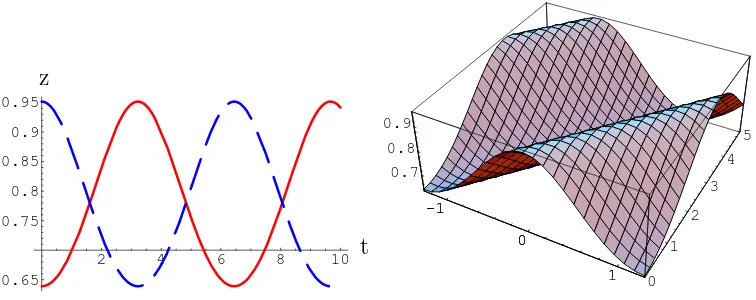
2 4 6 8 10 0.65
0.75 0.8 0.85 0.9 0.95 z
t
-1
0
1 0
1 2
3 4
5
0.7 0.8 0.9
-1
0
[image:25.612.118.496.70.220.2]1
Figure 7: First picture: plot of the time evolution of the end point and middle point of finite J magnon in the z direction. The red (solid) line are string end points, while the blue (dashed) line is the middle point of the string. Plot is made forω = 1.3 and v= 0.4 Second picture: plot of time evolution of string in the z
direction; axis x=σ,z= cosθ,y-time.
an open string.7 For finiteE a justification to such a choice of boundary conditions
comes from the consideration of the string theory in the uniform gauget=τ where the world-sheet momentum (2.14) is equal to the change of ∆x− = ∆φ. One can see that these boundary conditions are compatible with the equations of motion and Virasoro constraints.
The finite E solution can be easily found by introducing a “light-cone” coordi-nate ϕ
ϕ =φ−ωt , (5.7)
and taking the same one-soliton ansatz which was used in section 2
ϕ =ϕ(σ−vωτ), z =z(σ−vωτ). (5.8)
Note that the velocity of the soliton in the conformal gauge is vcg = vω. We use
this parametrization because, as we will see in a moment, the parameters ω and v
coincide with the corresponding parameters in thea= 0 uniform gauge. Recall that the parameter ω should be greater than 1, and go to 1 as E approaches infinity, as can be also seen by analyzing the folded string solution of [15], andv2 <1/ω2.
For our ansatz the Virasoro constraints give the following equations
ϕ′ = vω
2
1−ω2v2
z2−z2
min
1−z2 , (5.9)
z′2 = ω
2
(1−ω2v2)2 z 2−z2
min
z2max−z2
, (5.10)
7Let us note that the nonperiodicity ofφ(up to a winding number) is the reason why the giant
-1
0
1 0 1
2 3
4 5
-4 -3 -2 -1
0
-1
0
[image:26.612.183.432.65.272.2]1
Figure 8: Plot of time evolution of string in φ direction; axis are labeled as:
x=σ,z=φ,y-time (parameters areω= 1.3 and v= 0.4).
where
z2min = 1− 1
ω2 , z 2
max = 1−v2. (5.11)
We see that for this solution the derivativez′ is finite everywhere, and vanishes both
forz =zmax andz =zmin. This derivative, however, does not have a gauge-invariant
meaning. The real target-space shape of the solution is determined bydz/dϕ, which vanishes at z = zmax but diverges at z = zmin. The derivative is in fact equal to
the derivative dz/dx− (3.14) in the a = 0 uniform gauge, and it is clear, therefore, that this configuration is the same as the one we studied in section 2, see Fig.(6). In particular, one of the parameters of the solution, for example ω can be determined from the periodicity condition for z which takes the same form as equation (3.10). The velocity v can then be expressed in terms ofpby using the boundary condition (5.6) for φ and takes the following form
p= Z r
−r
dσ φ′ = 2 Z zmax
zmin
dz ϕ′
|z′|. (5.12)
Since |ϕz′′| =pz fora= 0, see (3.13), the change of φ is just equal to the world-sheet momentumpws in the a= 0 uniform gauge. This is what one should expect because
we supplemented the conformal gauge by the condition t=τ. Finally, the chargeJ is found by using equation (5.5)
J =
√
λ π
Z zmax
zmin
dzω(1−z
2)(1−vϕ′)
5 10 15 20 t
-6 -4 -2 2 phi
5 10 15 20 t -0.5
[image:27.612.130.481.68.175.2]0.5 1 1.5 2 2.5 phi
Figure 9: Left plot: A time evolution of the end and middle points of finite J
magnon in ˜ϕdirection. Red and blue lines are string end points, while green line is the middle point of the string. Right plot: Motion of end and middle point after subtraction of the center of mass motion. Both plots are made for ω = 1.3 and v= 0.4
All these integrals can be easily computed in terms of elliptic functions by using formulas from Appendix B. Computing the integrals, we find that the soliton energy
E −J, charge J and momentum p are given by exactly the same formulas (B.4), (B.5) and (B.7) as in the a = 0 uniform gauge. Therefore, the dispersion relation in the conformal gauge has the same form as the one in the a = 0 gauge, and the leading and subleading exponential corrections to E−J are given by
E−J =
√
λ π sin
p
2 h
1− 4
e2 sin 2 p
2 e
−R− (5.14)
−4
e4 sin 2p
2
R2(1 + cosp) + 2R(2 + 3 cosp) + 7 + 6 cospe−2R+· · ·i,
where the effective length which measures the magnitude of the correction is
R= √2πJ
λsin p2 . (5.15)
The “half-GKP” solution again corresponds to the limit v →0 orp→π. The finite
J correction to the dispersion formula is of course given by the same equation (3.20).
In the conformal gauge case, it is not difficult to write down an explicit solution of equation (5.10) by using Jacobi elliptic functions
z =
√
1−v2
ω√η dn
1
√η√σ−vτ
1−v2, η
, (5.16)
where
η= 1−ω
2v2
Figure 10: Plot of the superposition ofN magnons with equal world-sheet mo-menta. The string is nonrigid. All the individual magnons are hopping in the same direction and with the same velocity. The left picture shows the configura-tion at t= 0, and the right one shows the configuration after one hop.
Figure 11: Plot of the N-magnon case: N∆φ = 2π. This is a legitimate closed string configuration. Closed string is rigid! We do not see hopping of the individual magnons any more because there are no end-points.
is an elliptic modulus which is determined by the periodicity condition. This formula allows one to understand easily the target space-time evolution of the soliton, see Fig.4 and the simulations at http://www.aei.mpg.de/~peekas/magnons/.
Let us discuss the geometry of the finiteJ magnon solution. The solution in the
z direction is clearly periodic, since it is proportional to Jacobi elliptic function dn (5.16). The motion of the end points (σ =±r) and of the middle point (σ = 0) is periodic with the period T = 2r/v, and is depicted as a function of time on figure (7).
We see that as ω → 1 (corresponding to the limit of infinite J), the period diverges, corresponding to the fact that it takes infinite amount of target space-time for the soliton to propagate from one end of the string to another, given the fact that “effective” string length is infinite in this limit.
sinθ= 1
ω sinθ=v
Equator
[image:29.612.213.420.64.216.2]∆ϕ
Figure 12: Plot of the N-magnon configuration: N∆φ= 2π.
Neumann boundary conditions for all times.
Motion in the ϕ direction is also non-trival as can be seen by (numerically) integrating equation (5.9). The time evolution of integrated expression for ϕ is shown on the left plot of figure (8). We see that in addition to the global motion
ωt, for finiteJ configuration, motion inϕ direction also contributes to the center of mass motion. Subtracting this contribution, we obtain the periodic motion depicted on the right hand side plot of figure (9).
Let us also mention that in the case when p = 2Nπ we can build a closed string configuration by gluingN finiteJ solitons, see Fig.(10), (11) and (12). The resulting configuration carries the charge NJ and was studied in [53].
6
Two-spin giant magnon
In this section we show that a 2-spin giant magnon configuration recently discussed in [39] can be easily obtained by “boosting”8 a giant magnon in an orthogonal
direction in the same way as the usual 2-spin folded string solutions were found [16]. For simplicity we restrict our consideration to the conformal gauge and infinite J
case but similar solutions exist also in a unitary gauge and for finite J. The finite
J 2-spin solution in the conformal gauge is briefly discussed in Appendix D. The action for strings in R×S
3 is the sum of the action (5.2) for strings in
R×S
2
and a term depending on the angle α parametrising the second isometry direction of S3:
S =− √
λ
4π
Z r
−r
dσdτ
∂µz∂µz
1−z2 + (1−z 2)∂
µφ∂µφ+z2∂µα∂µα
, (6.1)
8
and we also impose the Virasoro constraints
˙
z2+z′2
1−z2 + (1−z
2)φ˙2+φ′2+z2 α˙2+α′2
= 1, (6.2)
˙
zz′
1−z2 + (1−z
2) ˙φφ′+z2αα˙ ′ = 0. (6.3)
The two charges J1 ≡J and J2 corresponding to shifts of φ and α are
J =
√
λ
2π
Z r
−r
dσ(1−z2) ˙φ , (6.4)
J2 =
√
λ
2π
Z r
−r
dσ z2α .˙
In the infinite J case we can look for soliton solutions of the form
z =z(σ−vτ), φ=ϕ(σ−vτ) +τ , α=ντ −νvσ . (6.5)
The first termντ in the ansatz forαdescribes the motion along the circle parametrized by α. It appears because we boost the infinite J giant magnon in the direction parametrized by α. One can easily check, however, that the equation of motion for
α forces us to add the second term proportional to σ.
Substituting the ansatz (3.5) in the Virasoro constraints (6.2), we get
ϕ′ = v
1−v2
z2
1−z2 , (6.6)
z′2 = z2 (1−v
2)(1−ν2(1−v2))−(1−ν2(1−v2)2)z2
(1−v2)2 . (6.7)
The solution to equation (6.7) is
z = ζ
cosh(γ(σ−vτ)), (6.8)
where the parameters ζ and γ are defined as follows
ζ = s
(1−v2)(1−ν2(1−v2))
1−ν2(1−v2)2 , γ =
r
1−ν2(1−v2)
1−v2 .
Note that the parameters satisfy the identity γ
√
1−ζ2
ζ =
1−v2
v2 .
The solution (6.8) can be easily used to computep, J2 and E −J. We obtain
p = 2 arcsinζ ,
J2 =
√
λ π ν
ζ2
γ ,
E−J =
√
λ π
ζ2
Finally, taking into account the identity ν2+γ2
ζ2 =
1
(1−v2)2 ,we obtain the dispersion relation for the 2-spin magnon
E−J = r
J2 2 +
λ π2 sin
2 p
2. (6.9)
The solution and the dispersion relations coincide with the ones found in [39] by using a rather non-trivial relation of the string sigma model on R ×S
3 with the
complex sine-Gordon equation. Our approach can be easily generalised to find a 3-spin giant magnon configuration.
Acknowledgments
We are grateful to R. Janik, J. Maldacena, K. Peeters, J. Plefka, M. Staudacher and A. Tseytlin for useful discussions. Special thanks to K. Peeters for helping us to make the giant worms animation. This work was supported in part by the grant
Superstring Theory (MRTN-CT-2004-512194). The work of G. A. was supported in part by the RFBI grant N05-01-00758, by NWO grant 047017015 and by the INTAS contract 03-51-6346.
A
Some explicit formulas
Here we present explicit expressions for the formulas from section 3 and specify them to the three simplest cases a= 0,1/2,1.
The density of the gauge-fixed Hamiltonian H appearing in (3.4) as a function of the coordinate z and the momentum pz canonically conjugate to z is
H = − 1−(1−a)z
2
1−2a−(1−a)2z2 (A.1)
+ p
1 + (1−z2) (1−2a−(1−a)2z2)p2
z p
1−z2+ (1−2a−(1−a)2z2)z′2
1−2a−(1−a)2z2 ,
The density of the Hamiltonian (A.1) for the three simplest cases:
a= 0 : H = −1 + r
1 +z′2
1−z2
q 1 +p2
z(1−z2)
2
,
a = 1
2 : H = −2 +
4
z2 −
1
z2
p
4(1−z2)−z2z′2p 4−p2
zz2(1−z2),
a= 1 : H = 1− q
1−z2−(z′)2p1−(1−z2)p2
z.
Solving the equation of motion for pz following from the action (3.4), we determine
the momentum as a function of ˙z and z
pz =
˙
z
p
(1−z2)q(1−z2)2−(1−2a−(1−a)2z2) ˙z2−(1−z2) (z′)2