Space translation properties and the minimum BER linear combiner DFE

S.Chen B. Mulgrew E.S. Chng G.J.Gibson

Indexuzg terms Bayesian equalisers, BLt evor rate, Equalisers, Decuion feedback equaliser

Abstract: Decision feedback in a decision feedback equaliser (DFE) performs a space translation that maps the DFE onto a transversal equaliser in the translated observation space. Properties of DFEs can therefore be analysed more easily by exploiting this geometric translation property. This approach is used to analyse the conventional DFE that employs a linear combination of the channel observations and the past decisions (the linear-combiner DFE). It is demonstrated that the usual minimum mean square error (MMSE) solution does not achieve the full performance potential of the linear- combiner DFE structure. A bit error rate (BER) expression for the linear-combiner DFE with binary signalling is obtained, and a method is proposed to optimally set the coefficients of the linear-combiner DFE. The performance of this minimum-BER (MBER) linear-combiner DFE is much closer to that of the optimal Bayesian DFE, compared with the MMSE linear-combiner DFE.

1 Introduction

Decision feedback is a powerful technique for combat- ing intersymbol interference (ISI) distortion. The con- ventional DFE [I] is based on a symbol-decision structure that employs a linear combination of the channel observations and the past decisions. We call this DFE the linear-combiner DFE, in contrast to other DFE structures that use nonlinear combinations of the channel observations and the past decisions [2-

61. One advantage of the linear-combiner DFE is its computational simplicity. The optimal solution for the symbol-decision structure with feedback is the Bayesian DFE 141. The adaptive Bayesian DFE has been shown

0 IEE, 1998

IEE Proceedings online no. 19982281

Paper first received 23rd December 1996 and in revised form 30th Sep- tember 1997

S. Chen is with the Department of Electrical and Electronic Engineering, University of Portsmouth, Anglesea Building, Portsmouth PO1 3DJ, UK B. Mulgrew is with the Department of Electrical Engineering, University of Edinburgh, Kmg’s Buildings, Edinburgh EH9 3JL, UK

E.S. Chng is with the Institute of Systems Science, National University of Singapore, Singapore 119597

G.J. Gibson is with Biomathematics & Statistics Scotland, James Clerk Maxwell Building, Kmg’s Buildings, Edinburgh EH9 3JL, UK

to outperform the adaptive maximum likelihood sequence estimator (MLSE) for severely fading mobile channels [7]. This is because the MLSE [8], although offering the best solution for equalisation under sta- tionary conditions, can suffer from the drawback of accumulating channel tracking errors under highly non- stationary environment. The Bayesian DFE can be viewed as a special case of the Bayesian sequence esti- mation [3, 91.

Previous research has demonstrated that decision feedback in

a

DFE translates the channel observation space (e.g. [3, lo]). In this paper we further investigate this geometric translation property and derive the explicit formula for performing this space translation. Viewed from the translated observation space, a DFE becomes a simpler transversal equaliser. Many proper- ties of DFEs can therefore be analysed more easily by considering their equivalent forms on the translated space. For example, by adopting this geometric approach, a concise form of the Bayesian DFE has been developed [ 1 11 which has certain advantages over the original form of the Bayesian DFE given in [4].

The Wiener or MMSE solution is often said to pro- vide the optimal solution for the coefficients of the lin- ear-combiner DFE. An elegant and rigorous analysis of the MMSE linear-combiner DFE is given in [12]. It is well known however that the MMSE solution does not necessarily correspond to the MBER solution, the BER being the ultimate performance criterion of equalisa- tion. Using the geometric translation approach it becomes obvious that the subsets of the translated channel states corresponding to different decisions are linearly separable. The linear-combiner DFE realises a linear decision boundary in the translated observation space. In the asymptotic case, where the signal-to-noise ratio

(SNR)

tends to infinity, the hyperplanes of the Wiener decision boundary are orthogonal to the last axis of the translated observation space. We demon- strate that the best

or optimal linear decision boundary

can be very different from the decision boundary of the Wiener solution.

Since the MMSE solution does not achieve the full performance potential of the linear-combiner DFE structure, a substantial BER reduction over the MMSE solution is possible by searching for a better solution of

the linear-combiner DFE. We derive a BER expression for the linear-combiner DFE with binary signalling. Using this BER estimator as the optimisation criterion, a method is proposed to optimally adjust the coeffi- cients of the linear-combiner DFE. The decision

boundary of this MBER linear-combiner DFE is the best linear approximation to the nonlinear Bayesian decision boundary. Adaptive implementation of this MBER linear-combiner DFE is also discussed. A draw- back of the MBER linear-combiner DFE is that the computational complexity increases significantly when extending to the multilevel signalling case.

Throughout this study the channel and the symbol constellation are assumed to be real valued. This corre- sponds to the use of multilevel pulse amplitude modu- lation (M-PAM) scheme. For the complex-valued channel and modulation schemes, the results

of the cur-

rent study are still valid [ 5 ] . Specifically, the channel is modelled as a finite impulse response filter with the transfer function

n, -1

A ( % ) = a& (1) i = O

where n, is the length of the channel impulse response and ai are the channel tap weights. The symbol sequence { s(k)} is independently identically distributed (IID) and has an M-PAM constellation defined by the set

s i x 2 i - M - 1 , l < i < M (2)

The received signal is given by

r ( k ) = ~ ( k )

+

e ( k ) =

n,-l

a i s ( k - i )

+

e ( k ) (3)

where V(k) is the noiseless channel observation, e(k) is an IID gaussian noise source with zero mean and vari- ance E[e2(k)] = 0: and is uncorrelated with s(k), and

E[.] denotes the expectation operator. The SNR

of

the system is defined as

S N R = E [.2(k)] / E [ e 2 ( k ) ] = g:

(

a:) /oz

i=O

n,-1

i=O

(4) where 0; = E[s2(k)] is the symbol variance.

decision device filtering

r(k)l r(k-l)I r(k-m+l)l

'(k-d)

[image:2.612.64.277.394.569.2]

w -

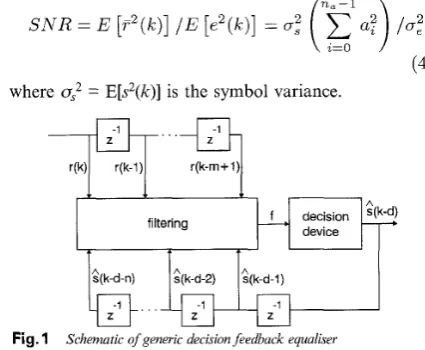
I

Fig. 1 Schematic of generic decision feedback equaliser

2

The structure of a generic DFE is depicted in Fig. 1. The equalisation process defined in Fig. 1 uses the information present in the observed channel output vector

Decision feedback as space translation

r(k) = [ r ( k ) . . . r ( k - m

+

t)]' ₍₅₎

and the past detected symbol vector

& ( k ) = [ i ( k

-

d

-

1 ) . . . i'(k - d - n)]' (6) to produce an estimate

d(k

-

4

of s(k -

d).

The integers d, m and n are known as decision delay, feedforward

I E E Proc.-Commun., Vol. 145, No 5, October 1998

order and feedback order, respectively. Without the loss of generality, d = n, - 1 is chosen to cover the entire channel dispersion,

m

is related to d by

m

= d

+

1 = n,, and

n

is given by n = n, + m - d - 2 = n, - 1.

We show that this choice of the DFE structure param- eters is sufficient to guarantee the linear separability of the subsets of the channel states related to the different decisions.

Applying the channel model (eqn. 3 ) to each element of the observation vector (eqn. 5) gives rise to

r(k) = F s ( k )

+

e ( k ) ₍₇₎

where e(k) = [e(k)

...

e(k - m

+

1)IT, s(k) = [sfT(k)

sbT(k)lT with

T } ( 8 ) S f ( k ) = [ s ( k ) . . . s ( k - d ) l T

sb(k) = [ S ( k - d - 1 ) .

. .

S ( k - d - n)]

and the m x (d

+ 1

+

n) matrix F has the form

F

=

[Fl

F 2 1 (9) with the

m

x (d

+

1) matrix Fl and m x n matrix F2 defined by

and

Fz =

respectively. Under the assumption that the feedback vector is correct, that is, Sb(k) = sb(k), eqn. 7 can be rewritten as

r(k) =

F I s f ( k )

+

F2&,(k)

+

e ( k ) (12) Thus the original observation space r(k) is transformed into a new space r'(k) owing to decision feedback

r'(k) = r(k) -

F2sb(k)

₍₁₃₎

Furthermore, the elements of r'(k) can be computed recursively according to the formula

I

~ ' ( k - i ) = K I T ' ( & i

+

1) - an,-,?(k - d -

I),

i = m - 1,.

. .

, 2 , 1 ? - ' ( I C ) = r ( k )

(14) where 2-l should be interpreted as the unit delay opera-

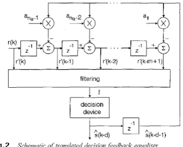
tor. Based on this interpretation of decision feedback, an alternative DFE structure is depicted in Fig. 2. A DFE is reduced to a transversal equaliser in the trans- lated space. Some researchers have realised this space translation nature of decision feedback [3, 101 but they did not go as far as to derive eqn. 14 and Fig. 2. Since the structure of Fig. 2 is equivalent to that of Fig. 1,

certain properties of a DFE can be studied by consider- ing its corresponding transversal equaliser, which is an easier task. This is the approach adopted in [ll] to derive a concise version of the Bayesian DFE. Iltis [13] has developed an importance sampling simulation tech- nique for evaluating the performance of the Bayesian

equaliser. This technique can readily be applied to eval- uate the lower-bound performance (with correct feed- back)

of the Bayesian DFE based on space translation.

“

.

.

‘

I

r’(k-1) r’(k-2) r’(k-m+ 1)

filtering

f

decision device

$k-d)

Fig. 2 Schematic of translated decision feedback equaliser.

We have the following result for the general DFE.

Let the Nf = Md+’ sequences or states of skk) be sJj for

1 s j 5 Nf. The set of the noiseless channel states in the translated space is

This set can be partitioned into M subsets conditioned on s(k -

d)

=

sI,

1 s i 5 M ,

a

R(’) = {ri E R’JS(/C - ci) =

s ’ } ,

₁ 5 _z

5

M

(16)

Result I : R(I), 1 5 i 5 M , are linearly separable. The proof of this result is given in the Appendix (Sec- tion 7.1). This result shows that the mapping Fl : r’ =

Fl sf maps linearly separable sets in the sfspace onto linearly separable sets in the r’-space. This is in contrast to the case of an equaliser without decision feedback where the mapping F : r = Fs maps a large space s onto

a

smaller space r. Hence states which are linearly sepa- rable in the s-space will not necessarily be linearly sepa- rable in the r-space (see appendix in [14]). Even though R(I), 1 s i 5

A4

are linearly separable, the optimal deci- sion boundary will generally be nonlinear (the Bayesian DFE). However, linear separability of the channel states related to the different decisions is a desired property to have because equalisation performance in this case is generally much better than that of the non- linear separable case.

We use a simple example to illustrate the space trans- lation property of decision feedback. Consider the channel

A1 ( z ) = 0.5

+

1 .O K 1

(17)

and the equaliser structure of d = 1, JW = 2 and M 1 1 .

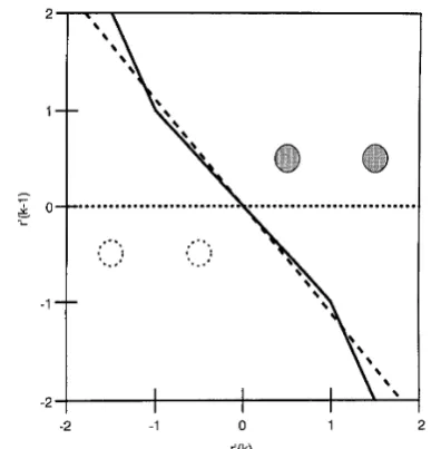
Assume that the symbol constellation is 2-PAM, that is, s(k) E 121). The set of the channel states in the orig- inal observation space r(k) is listed in Table 1 and depicted in Fig. 3. The decision feedback s(k - 2) corre-

sponds to a space translation, the effect of which is also illustrated in Fig. 3. It can be seen that decision feed- back effectively merges channel states and this simpli- fies the decision process. The two subsets of the translated states, the darkened states {dl, rr2} and {rf3,

rr4} in Fig. 3, are obviously linearly separable.

318

5 ’

-‘t

,--.. _.. , I

, ,

.. , ...’ s(k-2) = 1

translated

0

s(k-2)=-1

I 8 _I

I I I

-2 -1 0 1 2

r(k)+ r’(k)

Fig.3

states for chunnel Illustration Al(z) of effect = 0.5 t of I.0z-l decision feedback with a 2-PAM sjk constellation - 2) on channel

Table 1: Symbol and channel states for A,(z) 0.5

+

1 . 0 ~ ’ with 2-PAM constellation

NO. ~ ( k ) ~ ( k - 1) ~ ( k - 2 ) T(k) T ( k - 1)

1 -1 -1 -1 -1.5 -1.5

2 1 -1 -1 -0.5 -1.5

3 -1 1 -1 0.5 -0.5

4 1 1 -1 1.5 -0.5

5 -1 -1 1 -1.5 0.5

6 1 -1 1 -0.5 0.5

7 -1 1 1 0.5 1.5

8 1 1 1 1.5 1.5

3 Linear-combiner DFE

The linear-combiner DFE is based on a linear filtering of

r(k)

and s^b(k), and the decision is made by quan- tising the filter output

f ( r ( k ) , & , ( k ) ) = wTr(k)

+

b T g b ( k ) (18) where w = [wo ... wm-l]T and b = [b,

...

b,lT are the coef- ficients of the feedforward and feedback filters, respec- tively. Since the linear-combiner DFE is a special case of the generic DFE structure depicted in Fig. 1, by per- forming the translation of eqn. 13, it is reduced to the equivalent linear equaliser ‘without decision feedback’:

f’(r’(k))

= wTr’(k) (19)

The decision boundary of this equivalent linear equal- iser consists of M - 1 hyperplanes defined by: (r’ ; wTr’ = 2i - M } , 1 5 i 5 M ~ 1. These M - 1 parallel hyper-

planes can always be designed properly to separate the M subsets of the translated channel states 1 5 i s

M . In particular, for M = 2, the decision boundary, {r‘

: wTr’ = 0}, is a hyperplane passing through the origin of the r’(k)-space.

The Wiener or MMSE solution is often said to pro- vide the optimal w and b. It is however optimal only with respect to the mean square error criterion. Obvi- ously, there must exist a solution wept which achieves the best equalisation performance for the structure of eqn. 19. We refer to this wept as the MBER solution of the linear-combiner DFE. The MMSE linear-combiner DFE is generally not this MBER solution. A natural question is how different the MMSE and MBER solu- tions can be. We demonstrate that the performance gap between these two solutions can be large.

[image:3.613.334.534.46.210.2] [image:3.613.101.289.85.235.2] [image:3.613.326.542.261.392.2]

3.1

MMSE linear-combiner DFE

The MMSE solution for the linear-combiner DFE is well known [12]. Let w and

6

be the MMSE solution of

w and b. It can readily be shown that

[E]

=

[

-&]

where

and

c = 0; [ U , , - l an,-2

. . .

aO]* (21)

T = ( r -

Here

with

(24)

and 6(q) is the discrete Dirac delta function. Since wTF2 = -bT,

WTr(k)

+

IjT;b(k) = WTr'(k) ₍₂₅₎

It merely confirms the space translation nature of decision feedback. Thus, when examining the MMSE linear-combiner DFE we can simply study the feedfor- ward part of the solution. In the asymptotic case of SNR

-

to, we have the following result for

G.

Result 2: In the noise-free case

W = [ O 0

This result can be derived by setting

02

4 0 in eqn. 20.

However, an alternative proof is given in the Appendix (Section 7.1). In the limit case of SNR

-

to, the hyper-

planes of the MMSE solution are always orthogonal to the last axis of the r'(k)-space regardless of the channel. This cannot be the optimal solution for eqn. 19. Con- sider the example given in Table 1. The decision boundary of the Wiener solution for SNR

-

00 is

depicted in Fig. 4. The best possible linear decision boundary can easily be constructed for this example, and the MMSE solution in this case is far away from the best linear solution.

When the noise is added the hyperplanes of the MMSE linear decision boundary will rotate and are no longer orthogonal to the axis r'(k - d). For the range of

meaningful SNRs, however, the gap between the MMSE decision boundary and the best linear bound- ary can be large. Consider the example of Table 1 again. When SNR 4 0, the Wiener decision boundary

will rotate towards the line with a slope -2 (I?Jo/ivl = 2).

For SNR = 15dB, the Wiener decision boundary is the line with a slope of -0.28 but the best linear decision boundary obtained by minimising the BER has a slope

[image:4.613.315.509.42.244.2]

of -1.03. In general the MMSE solution is different from the MBER solution, and searching for the latter is worthwhile since the improvement in the BER per- formance over the MMSE solution can be substantial, at least for certain channels.

...

\

...

1

-2 -1 0 1 2

r"

Fig. 4 As mptotic decision bounduries corresponding to large SNR j o r

channel Al$j = 0.5 f I.Oz-' with 2-PAM constellation and decision fied- back.

~ optimal Bayesian

- - - - best linear approximation

. . . Wiener solution

3.2

MBER linear-combiner DFE

For the notational simplicity we restrict the discussion to the 2-PAM constellation. Let R+ and R- be the two subsets of the translated channel states R' correspond- ing to s(k - d) = 21, respectively. Since R+ and R- are

linearly separable, the results of Section 7.2 apply. Under the assumption of correct decisions being fed back, the BER of the linear-combiner DFE can be cal- culated using

N f I 2

2

P E ( w )

= -

Q

( E )

(27)

Nf

i = l C e

where

" 1

Q ( x ) = ~ exp

(-$)

dx

(28)

fi

and v is any point in the decision hyperplane. Since this hyperplane passes through the origin of the r'(k) space one can always choose v = 0. For the general M-PAM case, similar results can be derived but computation will increase dramatically as M increases.

It is obvious that the MMSE solution does not mini- mise PE(w). The optimal linear-combiner DFE should minimise the BER of eqn. 27. The following algorithm can be employed to obtain the optimal weight vector wOpf for the MBER linear-combiner DFE.

Algorithm 1

Step 1. Use a channel estimator to obtain a channel model and an estimate of the noise variance

Step 2. Compute the subset of channel states R+ and use the low noise Wiener solution (eqn. 26) as the ini- tial value w(0)

Step 3. Use the gradient algorithm

to optimise w, where is an adaptive gain.

The derivative of

Pdw)

with respect to w can be found in the Appendix (Section 7.2). The gradient algorithm (eqn. 30) is an offline optimisation procedure and does not involve any channel observation r'(k). Thus the algorithm 1 is suitable for application to stationary channels. For nonstationary channels it is desirable to update the weights after each new observation sample is taken, and the following recursive adaptive algorithm can be used to achieve this purpose.

Algovithm 2. At the sample k:

Step 1. Use the least mean square (LMS) algorithm to update the channel estimate a(k) = [ao(k) ...

~,,-~(k)]~

and a noise variance estimator to update 0,2(k)

Step 2. Compute the subset of the channel states R+(k) and the gradient dPdw(k - 1))idw

Step 3. Update the equaliser's weights according to

Computational complexity of the adaptive MBER lin- ear-combiner DFE is considerably more than that of the standard adaptive MMSE linear-combiner DFE. However, the performance gain justifies the increase in computation. Some of the channel states rll E R+ are far away from the decision boundary and contribute little to the performance criterion of eqn. 27. Computa- tional requirements of the MBER linear-combiner DFE can be reduced significantly by neglecting these states from the optimisation procedure with little per- formance degradation. For example, consider the case of Fig. 4. By just using the single state at (0.5, 0.5) in the optimisation, little performance degradation will occur, compared with using the full set R+ of the two states.

I '

I I I I I I I

I I I I I I

4 6 8 10 12 14 16 18

SNR, dB

Fig. 5

P A M constellation with detected symbols being Sed back

-0- MMSE DFE

-t- MBER D F E

-0- Bayesian DFE

Peformance comparison for channel A (z) = 0 5 f I 0z-' and 2-

3.3

Simulation study

Two examples were used to compare the MBER and MMSE solutions of the linear-combiner DFE. The optimal weight vector wept for the linear-combiner DFE was obtained using the gradient algorithm (eqn. 30).

320

The first example was the channel given in Table 1. The decision boundary of the MBER linear-combiner DFE is depicted in Fig. 4 under the title 'best linear approximation' to emphasise the fact that it is the best linear approximation to the optimal nonlinear Bayesian boundary. This example clearly demonstrates that the MMSE solution does not achieve the full performance potential of the linear-combiner DFE structure. Fig.

5

compares the BERs as a function of SNR with detected symbols being fed back for the Bayesian, MBER lin- ear-combiner and MMSE linear-combiner DFEs. For this example, the MBER linear-combiner DFE is far superior over the MMSE solution and is very close to the optimal nonlinear Bayesian solution.

The second example was a five-tap channel with the transfer function given by

A ~ ( z ) = 0.227

+

0 . 4 6 6 ~ ~ ~

+

0 . 6 8 8 ~ - ~

+

0 . 4 6 6 ~ ~ ~

+

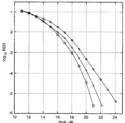
0 . 2 2 7 ~ ~ ~ ( 3 2 )

The structure of the DFE was chosen to be d = 4, m = 5 and n = 4. The BERs of the Bayesian, MBER linear- combiner and MMSE linear-combiner DFEs with detected symbols being fed back are plotted in Fig. 6,

where it can be seen that the performance of the MBER linear-combiner DFE is significantly better than that of the MMSE solution. The performance gap between the Bayesian DFE and the MBER linear-com- biner DFE confirms the fact that the real optimal solu- tion for the DFE structure of Fig. 1

is

generally nonlinear. The best linear solution is suboptimal in nature. However, the usual MMSE solution is inferior to this best linear solution.

-1

-2

LT

W m

0 -3

cn

-

-4

-5

-6 I 1 I I I I I

12 14 16 18 20 22 24

SNR, dB

Fi .6 Perfovmunce comparison for channel Az(z) = 0.227 + 0.4642-' f

0 . 8 E 2 t 0.461%~ + 0 . 2 2 7 ~ ~ and 2-PAM constellation with detected

svmbols being fed back

lo- MMSE~DFE

-+-

MBER DFE

-0- Bayesian D F E

The convergence behaviour of the algorithm 2 was tested using the following example. Initially, the chan- nel had a transfer function A3(z) = 0.8

+ 0.82'

with SNR = 15dB. At the sample k = 0, the channel jumped to the transfer function A l ( z ) = 0.5 + I.OZ-~. The LMS algorithm was used to estimate the channel taps with an adaptive gain 0.1 and eqn. 31 was used to update the equaliser weights with q = 0.1. The trajectories of [image:5.613.334.535.382.579.2]

the channel estimates ao(k)/al(k) and the equaliser weights w,(k)/w,(k), averaged over 50 different runs, are plotted in Fig. 7. It can be seen that the conver- gence speed of this adaptive procedure is reasonable.

I I I I I I I I

0 20 40 60 80

samples

Trajectories of channel estimates imd equaliser weights for chan-

Fi .7

ne?AI(zj = 0.5 t 1.0~-I with 2-PAM constellation

Two lines indicate respective optimal values

4 Conclusions

The geometric translation property of the decision feedback in the DFE structure has been investigated in this paper. Basically, the decision feedback performs a space translation that maps the DFE onto an equiva- lent transversal equaliser in the translated observation space. In particular, viewed from the translated obser- vation space, the linear-combiner DFE is reduced to a simpler linear equaliser. We have shown that, in the translated observation space, the subsets of channel states corresponding to the different decisions are always linearly separable and, under very low noise conditions, the hyperplanes of the Wiener decision boundary are orthogonal to the last axis of the trans- lated space. This demonstrates that the MMSE solu- tion does not achieve the best possible performance of

the linear-combiner DFE structure. Based on a

BER

expression, a novel

MBER

linear-combiner DFE has been derived for 2-PAM constellation, which achieves the full performance potential of the linear-combiner DFE structure and offers the best linear approximation to the nonlinear Bayesian solution. This MBER linear- combiner DFE can be extended to the general M-PAM case but computational requirements will increase sig- nificantly as M increases.

5 Acknowledgment

GJG acknowledges financial support from the Scottish

Office Agriculture, Environment and Fisheries Depart- ment.

6 References

1 QURESHI, S.U.H.: ‘Adaptive equalization’, Proc. IEEE, 1985, 2 SIU, S., GIBSON, G.J., and COWAN, C.F.N.: ‘Decision feed-

back equalisation using neural network structures and perform- ance comparison with the standard architecture’, IEE Proc. I, Commun. Speech Vis., 1990, 137, (4), pp. 221-225

3 WILLIAMSON, D., KENNEDY, R.A., and PULFORD, G.W.: ‘Block decision feedback equalization’, IEEE Trans. Commun.,

1992, 40, (2), pp. 255-264

73, (9), pp. 1349-1387

IEE Proc.-Commun., Vol. 145, No. 5, October I998

~

4

5

6

I

8

9

10

11

12

13

14

7

7.

~

Consider the matrix Fl which maps the m-dimensional space sf onto the m-dimensional space r’

r f = F I S ~ ( 3 3 )

(34)

The hyperplane in the sfspace

W T S f = 2i - M

divides the set of all sxj into two disjoint sets, where 1 5

i 5 M ~ 1. The decision metric for an sf2 in the set {sJj : 0 < wSTsf2 ~

(2i

-

M>>

is

d j =

w T s ~ , ~

- (22 -

M )

_{( 3 5 )}

Since PI is

a

square upper triangular Toeplitz matrix, its eigenvalues are its diagonal elements which are all

ao. Thus Fl is full rank and its inverse always exists. Let r> = F, sx]. Then sxl = F1-lr> and we write the deci- sion metric in terms of rri:

dJ = wFFclri - ( a i - M ) = wTrj - (22 - M ) (36)

where

w = F c T w , ( 3 7 )

Therefore we operate on the r’-space and produce the same decision metric. Hence if we start with linearly separable states in the sfspace, the states after the map- ping are also linearly separable in the r‘-space.

The set {sxj : s(k -

d)

> xi} is linearly separable from the set { s f i : s(k ~

d,

5 si}, where si is defined in eqn. 2,

since a suitable set of m weights that define the separat- ing hyperplane can be chosen as

w s = [ 0 0 - . . 0 1 ] T ( 3 8 )

Thus the two

sets

{R(O, 1 s 1 5 i} and {R(n, i

+

1 5

I

s

M } in the r’-space are also linearly separable, and the weight vector of the separating hyperplane is

w

= F T T I O

0 . ‘ . 0 1IT (39)

321 CHEN, S., MULGREW, B., and McLAUGHLIN, S.: ‘Adaptive Bayesian equaliser with decision feedback‘, IEEE Trans. Signal

CHEN, S., McLAUGHLIN, S., and MULGREW, B.: ‘Complex- valued radial basis function network, Part 11: application to dig- ital communications channel equalisation’, EURASIP Signal Process. J., 1994, 36, pp. 175-188

CHA, I., and KASSAM, S.A.: ‘Channel equalization using adap- tive comdex radial basis function networks’. IEEE J. Sel. Areas P ~ o c ~ L s . , 1993, 41, (9), pp. 2918-2927

Communr, 1995, 13, (l), pp. 122-131

CHEN, S., McLAUGHLIN, S., MULGREW, B., and GRANT, P.M.: ‘Adaptive Bavesian decision feedback equaliser for disoer- sive mobileAradio clknnels’. IEEE Trans. Commun.. , 1995. , 43.’(5). , ~ , ,

pp. 1937-1946

FORNEY, G.D.: ‘Maximum-likelihood sequence estimation of digital sequences in the presence of intersymbol interference’, IEEE Trans., 1972, IT-18, ( 3 ) , pp. 363-378

ABEND, K., and FRITCHMAN, B.D.: ‘Statistical detection for communication channels with intersymbol interference’, Proc. IEEE, 1970, 58, (5), pp. 779-785

CLARK, A.P., LEE, L.H., and MARSHALL, R.S.: ‘Develop- ments of the conventional non-linear equaliser’, IEE Proc. F, Commun. Radar Signal Process., 1982, 129, (2), pp. 85-94 CHEN, S., McLAUGHLIN, S., MULGREW, B., and GRANT, P.M.: ‘Bayesian decision feedback equaliser for overcoming co- channel interference’, IEE Proc. Commun., 1996, 143, (4) pp. 219- 225

C O F F I , J.M., DUDEVOIR,,G.P., EYUBOGLU, M.V., and FORNEY. G.D.: ‘MMSE decision-feedback eaualizers and cod- ing - part I: equalization results’, IEEE Trans: Commun., 1995,

43, (lo), pp. 2582-2594

ILTIS, R.A.: ‘A randomized bias technique for the importance sampling simulation of Bavesian eaualizers’, IEEE Trans. Com- mu;, 1!i95, 43, (2/3/4), pp. i 107-1 1 i5

GIBSON, G.J., SIU, S., and COWAN, C.F.N.: ‘The application of nonlinear structures to the reconstruction of binary signals’,

IEEE Trans. Signal Process., 1991, 39, (8), pp. 1877-1884

Appendix

Since Fl is upper triangular with all the diagonal ele- ments being ao, Fl-I is lower triangular with all the diagonal elements being l/ao. Hence

w = [ O 0 ’ . ’ 0

(40)

Notice that the weight vector (eqn. 40) is in fact the Wiener solution for the linear-combiner DFE in the case of zero noise. Let i = 1, ..., M - 1, we conclude

that R(0, 1 5 I s M , are linearly separable.

7.2

BER of linear equaliser f(r(k))

=

wTr(k)

for

2-PAM constellation

There are two subsets of the channel states

R+

and

R-

related to s(k ~

d)

= -cl, respectively. Let Z+ and

2-

be

the regions of r(k) related to the decisions s^(k ~

d)

= 21, respectively. The BER is given by

P Z

J’

pr(r~rt)dr+

c

~j

/

pr(rlrj)dr

PE =

r , E R + rEz.- r 2 E R - r E Z +

(41)

where pT(r(k)lrJ is the probability density function

(PDF) of r(k) conditioned on the received channel state being ri and

pi

is the a psiosi probability of ri. Let the number of the channel states be N,. For the symmetric and IID symbol constellation,

pi

= UN, and eqn. 41 is reduced to

N s / 2

2

P E = -

Pe(ri),

ri E Rf (42)

N s 2 = 1

where

Pe (ri) = pr(rlri)dr, ri E

R+

(43)

is the conditional error probability when the received channel state is ri E

R+.

When the two subsets R+ and R- are linearly separa- ble, that is

R+

and R- can be separated by the decision hyperplane wTr = 0, the BER expression can further be simplified. An orthogonal transformation x = Lr can be constructed which rotates the bases so that one of the transformed bases, say xI, is parallel to w, the

normal of the decision hyperplane. Since

LLT

= I and the noise e(k) has an IID gaussian PDF, the condi- tional error probability (eqn. 43) is reduced to

E ( r z ) =

TPz(xddxl~Pz(x2)dx2.f.

7

Pz(zm)dzm

P% --w --w

00

1

exp

(-5)

dx

2

Q

(E)

P%

(44)

where

(45)

is the euclidean distance between ri and the decision hyperplane, and v is any point in this hyperplane. The BER of the linear equaliser in this case can be expressed as

Here we have included w in the expression to empha- sise that for a given channel the BER depends on the equaliser weights. The derivative of P,(r,) with respect to

wj

is

x [(v - r z ) T ~ I I ~ / I - 3 w 3 -

I I w I I - ~ ( ~ ~

- r t 3 ) ]

(47)

O < J < m - l

where sgn(.) is the signum function,

vj

and r2/ are thejth elements of v and r,, respectively. The derivative of PE(w) with respect to

w3

is then given by