Abstract—Researches on supersonic ejector for refrigeration
application is increasingly becoming very attractive due to its simplicity and significant reduction in overall cost. However, most of the studies are still limited to one-dimensional mathematical modelling and physical experimentation. Data acquisition from physical investigations requires extensive effort and considerable time and is very expensive; whereas, Computational Fluid Dynamics (CFD) could be a more efficient diagnostic tool for ejector design analysis and performance optimization than one-dimensional mathematical modelling prior to actual experimentation. This study presents CFD simulation results of an ejector for air conditioning applications using popular commercial CFD software and attempts to have a highly dependable simulation that features a model based on the interpolation of real fluid properties from NIST-REFPROP database embedded through user-defined functions (UDF’s) with R134a as the working fluid. Primarily, density and speed of sound are polynomial functions of both pressure and temperature. In addition, a comparison is made between the results of the said model with that of the ideal gas model, which is one of the conventional models employed in dealing with compressible flows inside ejectors.
Index Terms—computational fluid dynamics, refrigeration,
supersonic ejector, user-defined function
I. INTRODUCTION
HE low-grade thermal energy such as waste heat from industrial processes and equipment, internal combustion engine exhaust heat, geothermal energy and solar energy can
Manuscript received March 20, 2017; revised April 10, 2017. The dissemination of this research is sponsored by the Engineering Research and Development Program (ERDT) of the Department of Science and Technology (DOST) of the Republic of the Philippines. The program is being managed and implemented by the College of Engineering of University of the Philippines–Diliman.
J. Honra is with the School of Mechanical and Manufacturing Engineering, Mapua Institute of Technology, Intramuros, Manila, 1002 Philippines (phone: +63-905-392-9814, +63-2-247-5000 loc 2105; e-mail: [email protected]).
M. S. Berana is with the Department of Mechanical Engineering, College of Engineering, University of the Philippines – Diliman, Quezon City, 1101 Philippines (phone: +63-915-412-0022, +63-2-981-8500 loc 3130; fax: +63-2-709-8786; e-mail: [email protected]).
L. A. M. Danao is with the Department of Mechanical Engineering, College of Engineering, University of the Philippines – Diliman, Quezon City, 1101 Philippines (phone: +63-949-184-7572, +63-2-981-8500 loc 3130; fax: +63-2-709-8786; e-mail: [email protected]).
M. C. E. Manuel is with the School of Mechanical and Manufacturing Engineering, Mapua Institute of Technology, Intramuros, Manila, 1002 Philippines (phone: +63-947-956-1459, +63-2-247-5000 loc 2105; e-mail: [email protected]).
be tapped as heat sources to power an ejector refrigeration system. This refrigeration system uses an ejector and a liquid pump in lieu of the electricity-driven compressor in conventional vapor compression refrigeration system. The liquid pump typically consumes only 1% of the heat input to the ejector system from low-grade heat sources or approximately 16-19% of the electricity consumption of the compressor in conventional system, given the same refrigerating capacity [1]. This translates to enormous potential savings in energy consumption when ejector refrigeration technology becomes mature and fully developed for commercial and industrial applications.
II. THEORY A. Ejector Theory
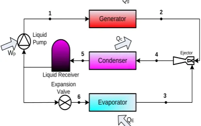
Ejector refrigeration system uses an ejector, a liquid pump and a vapor generator to replace the mechanical compressor. Fig. 1 illustrates a simple ejector refrigeration system with its major components labelled. The generator receives heat from a low-cost, low-grade thermal energy source and heats up the refrigerant to produce high pressure and high temperature vapor known as the primary fluid that enters the ejector and accelerates through the ejector nozzle where the jet issuing from it entrains the low-pressure secondary flow coming from the evaporator. The resulting fluid mixture which is at an intermediate pressure passes through the condenser, where heat rejection process occurs, and leaves as liquid refrigerant. Most of the refrigerant leaving the condenser is pumped back to the generator and the rest enters the expansion valve to reduce its pressure down to that of the evaporator where another heat absorption process takes place.
CFD Analysis of Supersonic Ejector in Ejector
Refrigeration System for Air Conditioning
Application
Jaime Honra, Menandro S. Berana, Louis Angelo M. Danao, and Mark Christian E. Manuel
T
Generator
Condenser
Evaporator Liquid Receiver
Liquid Pump
Ejector
Expansion Valve
Qg
Qc
QE Wp
3 2
4 1
5
6
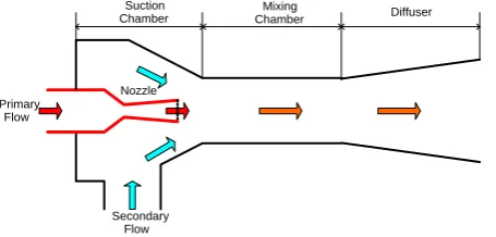
[image:1.595.319.527.636.766.2]One of the major parts of ejector is the converging-diverging nozzle as shown in Fig. 2. Primary fluid enters the nozzle at subsonic speed and leaves at supersonic condition with increased kinetic energy at the expense of pressure. The resulting difference in pressure between the nozzle exit and the secondary fluid inlet creates the entrainment effect where secondary fluid is sucked from the suction chamber. The mixture flows through the mixing chamber at constant pressure until it reaches the diffuser at subsonic velocity. The mixture is recompressed to the desired condenser pressure as it passes through the diffuser.
The system’s performance is best described by its Coefficient of Performance (COP) and the ejector’s entrainment ratio (ER). Mathematically, they are defined as,
(1)
(2)
B. Computational Fluid Dynamics (CFD) Theory The governing equations for fluid flow such as equations for conservation of mass, momentum, and energy form a set of coupled, nonlinear partial differential equations. Analytical methods may not be possible to solve these equations for most engineering problems, but, computational fluid dynamics is capable of dealing with these types of equations. CFD is a branch of fluid mechanics and is the science of predicting fluid flow, heat and mass transfer, chemical reactions, and related phenomena [2]. Its core part is the solver that uses a numerical calculation scheme. The domain is discretized into finite sets of control volume where the equations in the form of Navier-Stokes partial differential equations are solved. These equations are converted into a set of algebraic equations at discrete points which are then solved numerically to render a solution with the appropriate boundary conditions. The postprocessor gives the calculated results into convenient formats, either graphically or numerically. Fluid flow through the ejector can be considered compressible, turbulent, steady-state and axisymmetric. The Navier-Stokes continuity, momentum and energy equations provide the foundation in CFD simulation of fluid motion. The average values of flow quantities including velocity are usually determined by time averaging over large intervals, sifting out small variations, but small enough to maintain large scale time variations. This results in Reynolds-averaged Navier-Stokes (RANS) equations. To find closure to this, a popular approach to turbulence modelling employs the Boussinesq hypothesis to relate the Reynolds stresses to the mean velocity gradients [2], [3]. The subsequent equations are written in Cartesian tensor form as: (3)
(4)
(5)
(6)
The stress tensor and energy equations are given in equations 5 and 6, respectively. The total energy equation takes into account the effects of viscous forces on fluid motion as this incorporates the viscous dissipation in it.
III. EJECTORMODELLING A. Ejector Geometry
Ejector, being the most critical component dictates the overall performance of the ejector refrigeration system. Thus, its configuration and geometry must be carefully determined and designed. Initially, recommended ejector dimensions from ASHRAE and ESDU and non-dimensional parameters for ejector configuration from published journals are followed [4]-[9]. Combinations of such dimensions and parameters are tried on in the CFD simulation one by one until near-optimum geometry is established which gives maximum entrainment ratio at the desired operating conditions of the refrigeration system for R134a refrigerant. Table 1 gives the acquired specifications for the ejector geometry. Nozzle Primary Flow Secondary Flow Suction Chamber Diffuser Mixing Chamber
Fig. 2. Basic Ejector Geometry.
p s p g E m m ER W Q Q COP
j ij i j i j i i ix
x
p
u
u
x
u
t
u
x
t
0
ij k k eff i j j i eff ijx
u
x
u
x
u
[image:2.595.312.541.104.293.2]
3
2
ij j i eff i iu
x
T
P
E
u
x
E
t
.
TABLE IEJECTOR GEOMETRY SPECIFICATION Nozzle Inlet Diameter 10 mm
Throat Diameter 2.24 mm
Nozzle Exit Diameter 3.65 mm Nozzle Converging Angle 60° Nozzle Diverging Angle 10°
Suction Diameter 32 mm
Suction Converging Angle 42 ° Distance of Nozzle from
Mixing Section 5 mm
Mixing Section Diameter 5.1mm Mixing Section Length 39 mm Diffuser Outlet Diameter 13.84 mm
Diffuser Length 50 mm
Diffuser Angle 5 °
Total Ejector Length 108.24 mm Mixing section Length to
Diameter Ratio 7.6
Nozzle Exit Diameter to
[image:2.595.54.282.202.311.2]B. CFD Implementation
Two-dimensional (2-D) axisymmetric model of the flow domain is used to minimize computational time. Quad mesh is employed using Ansys Meshing due to geometric simplicity; and is imported to Ansys Fluent v.14.5, for mesh checking and subsequently, for the simulation. Temperature gradient adaptation is set to automatically refine meshes at regions where large temperature differences exist. This helps prevent diverging solution and makes the simulation process smooth. In addition, solver selected is density-based type with implicit formulation on the account that the flow is compressible. This type of solver computes the governing equations of continuity, momentum, and energy and species transport simultaneously; and afterwards, governing equations for additional scalars such as turbulence will be solved sequentially. For steady-state assumption with travelling shocks, implicit formulation may be more efficient. Although steady-state is applied, from the standpoint of numerical solutions, the unsteady term is conserved and governing equations are calculated with a time-marching technique. Convective transport variables are discretized using third-order MUSCL; while, the discretized system is solved with Least Squares Cell-based gradient calculations. Finally, Shear-Stress Transport (SST) k-ω turbulence model is used which takes into consideration the transport of the turbulent shear stress. This is the most recommended turbulence model for turbulent compressible flows [10], [11]. Single-phase flow assumption is considered since both flow inlet conditions are in the vapor states; although phase change can happen, it is likely to exist temporarily in small local regions and can be negligible. Boundary Conditions
In this CFD analysis, the fixed ejector geometry used is intended for an ejector refrigeration system for air-cooled air-conditioning applications for specific on-design operating conditions suitable for tropical countries like the Philippines, as follows: evaporator temperature, 10°C; condenser temperature, approximately 40°C and generator temperature, 95°C. The same geometry will also be evaluated at off-design conditions by varying the generator, condenser and evaporator temperatures (Tg, TC, TE) at ranges
90-95°C, 40-42°C, and 5-15°C, respectively. Pressure boundary conditions are imposed for both primary and secondary flows as well as at the diffuser outlet.
Real Fluid Properties
The approach is mainly concentrated on the calculation of density and speed of sound as polynomial functions of pressure and temperature to nearly depict properties of the refrigerant as prescribed by NIST-REFPROP [12]. User-defined function is formulated to incorporate density and speed of sound computations in the CFD platform. Thermal conductivity and viscosity are essentially made polynomial functions of temperature only, as their variations with temperature are generally found to be of negligible effects. Specific heat is largely linear with temperature, but the relationship varies at relatively small ranges of temperature to accurately predict the properties stipulated in the NIST
REFPROP database.
Ideal Gas Model Properties
The simplest equation of state that relates pressure, temperature and molar or specific volume is the ideal gas law. This equation which is approximately valid for the low- pressure gas regions is given as,
(7)
IV. RESULTSANDDISCUSSION
For the given on-design conditions for both inlets, the analysis predicts a back pressure or condenser pressure, PC=1,041,262 Pa, which corresponds to a desired saturation
temperature, TC =314.05 K (40.9°C). The entrainment ratio
and exit temperature are 0.30201 and 343.2 K, respectively. This indicates that the exit state is superheated. The computational domain consists of approximately 12,700 elements where very few of them fall within the mixture region, as plotted in the Fig. 3. Similar pattern also happens for ideal gas assumption. Thus, from a statistical point of view, the flow is basically single phase.
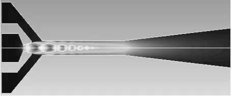
The contours of the velocity magnitudes illustrated in Fig. 4 reveals a near optimal ejector operation as the profile describes the existence of a series of oblique shock waves for the primary fluid downstream the nozzle exit and a weak
T
M
R
P
w
[image:3.595.304.543.380.571.2]
Fig. 3. Pressure-Temperature Plot of Computational Elements.
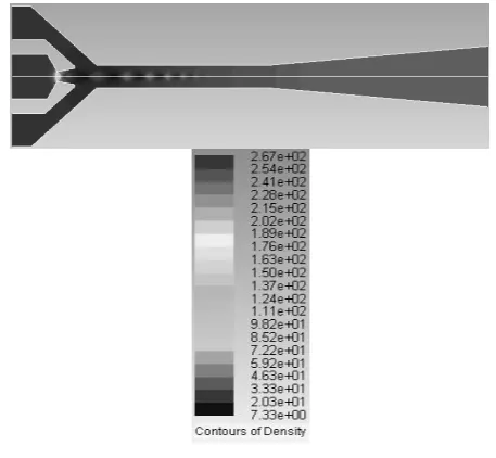
[image:3.595.318.546.608.703.2]single shock wave of the mixture flow at the diffuser inlet [13], [14]. This renders effective recompression of the fluid to the required diffuser outlet pressure, PC. The occurrence
of shock train is also visible in the outline of pressure profile in Fig. 5 and density profile in Fig. 6. Shock waves are characterized by abrupt changes in pressure with variation in densities. The predicted densities and speeds of sound are accurate within 96% confidence level; while, specific heat, viscosity and thermal conductivity are at 95% confidence level. Table 2 compares the resulting properties with the values from NIST-REFPROP [12].
The effects of varying inlet and outlet conditions are also evaluated with results shown in Tables 3 to 5. Increasing the outlet pressure results in decreasing entrainment ratio and consequently, decreasing the COP of the refrigeration system. Decrease of secondary pressure at lower TE and
reduction in primary pressure at lesser Tg, likewise lead to
diminishing entrainment ratio. The latter also results in some reverse flows through secondary inlet at Tg = 363.15 K,
which signifies ejector failure. It is also noteworthy that in Table 5, primary mass flow rate, mp drops due to insufficient
motive pressure to push the primary fluid through the nozzle throat.
The same fixed geometry is also utilized using the ideal gas model on the same on-design conditions; and the results are compared with the earlier simulation model. Table 6 shows the variation in the entrainment ratio, slight increase in diffuser outlet pressure and the difference in the outlet temperatures. The large deviation in the primary mass flow rates is due to the huge difference in the primary inlet densities. Higher density for the primary fluid results in greater amount of flow through the nozzle throat given the same cross-sectional area. This also causes more secondary TABLE II
COMPARISON OF SIMULATION RESULT AND NIST PROPERTY VALUES
Density, kg/m3 Speed of Sound, m/s
Result NIST Result NIST
[image:4.595.302.542.195.644.2]Primary Inlet 266.83929 267.14 102.96661 101.91 Secondary inlet 20.304201 20.226 146.4184 146.38 Diffuser Outlet 41.065052 42.452 157.42618 156
TABLE III
EFFECT OF INCREASING CONDENSER PRESSURE ON ENTRAINMENT RATIO
Boundary Conditions
PC, MPa TC, K mp, kg/s ms, kg/s ER
1 1.0166 313.15 0.051819 0.01565 0.30201
2 1.0441 314.15 0.051819 0.01170 0.22584
3 1.0722 315.15 0.051819 0.00777 0.14986
This is at constant primary and secondary inlet conditions: Pg=3.5912 MPa at Tg =368.15K and PE=0.41461MPa at
TE=283.15 K
TABLE IV
EFFECT OF DECREASING EVAPORATOR PRESSURE ON ENTRAINMENT RATIO
Boundary Conditions
PE, MPa TE, K mp, kg/s ms, kg/s ER
1 0.41461 283.15 0.051819 0.01565 0.30201
2 0.38761 281.15 0.051819 0.01275 0.24607
3 0.37463 280.15 0.051819 0.01163 0.22448
4 0.36198 279.15 0.051819 0.01045 0.20156
5 0.34966 278.15 0.051819 0.00913 0.17624
6 0.33766 277.15 0.051819 0.00776 0.14966
This is at constant primary inlet and diffuser outlet conditions: Pg=3.5912 MPa at Tg =368.15K and PC=1.0166 MPa at
TC=313.15 K
TABLE V
EFFECT OF DECREASING PRIMARY PRESSURE ON ENTRAINMENT RATIO
Boundary Conditions
Pg, MPa Tg, K mp, kg/s ms, kg/s ER
1 3.5912 368.15 0.051819 0.01565 0.30201
2 3.5193 367.15 0.050890 0.01322 0.25985
3 3.4487 366.15 0.049922 0.01124 0.22511
4 3.3793 365.15 0.048942 0.00909 0.18563
5 3.3112 364.15 0.047961 0.00676 0.14104
6 3.2442 363.15 0.046977 0.00446 0.09498
This is at constant secondary inlet and diffuser outlet conditions: PE=0.41461MPa at TE=283.15 K and PC=1.0166 MPa at
TC=313.15 K
[image:4.595.55.277.203.393.2]Fig. 5. Contours of Pressure in Pa
[image:4.595.53.282.439.650.2]fluid entrainment that tends to increase the entrainment ratio and the refrigeration system’s COP. In the first simulation the primary fluid density at inlet is 266.84 kg/m3 while for
the ideal gas, it is only 119.71 kg/m3.
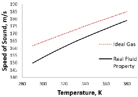
For further comparison of the two (2) models, Fig. 7 illustrates the functional relationship of density at varying temperatures given a constant pressure. Also Fig. 6 shows speed of sound, which largely depends on the density particularly for the real fluid property, as function of temperature at constant pressure. For real fluid property, both density and speed of sound are polynomial functions of temperature at a given pressure, that is, density increases more rapidly with the decrease in temperature and as the temperature reduces the speed of sound decreases at a faster rate. In ideal gas model, both density and speed of sound almost vary directly with temperature.
V. CONCLUSION
At specific refrigeration operating conditions, there is a corresponding ejector of fixed configuration that will operate at optimal condition. In this study, a fixed-geometry ejector is determined for the given on-design conditions that works on a near optimal ejector operation. A near optimal ejector operation is characterized by a number of oblique shocks that gradually fades into a weak shock at the end of the mixing section for an effective recompression. Over-expansion and under-Over-expansion of the jet coming from the nozzle indicate ineffective recompression and lower entrainments, respectively. The Real Fluid Property simulation predicts more accurately the thermodynamic properties prescribed in the NIST-REFPROP Database than the Ideal Gas Model. The former also gives higher entrainment ratio and COP, thus, it can be considered a more reliable approach. However, such advantages cannot be construed to say that one model is better than the other unless an experimental validation is done in the future to further verify this claim.
NOMENCLATURE
CFD Computational Fluid Dynamics (-) COP Coefficient of Performance (-) ER entrainment ratio (-) E Total Energy (J) mass flow rate (kg/s) Mw Molecular weight (kg/kmol)
P pressure (Pa) Q heat (W) RANS Reynolds-averaged Navier-Stokes (-) R Universal Gas Constant (J/kmol-K) T temperature (K) UDF User-defined Function (-) ρ density (kg/m3)
ui velocity (m/s)
stress tensor (-) x, y, z coordinates (-) α thermal conductivity (W/m-K) μ dynamic viscosity (kg/m-s) k turbulent kinetic energy (J) δij Kronecker symbol (-)
Subscripts
C condenser
E evaporator
eff effective
g generator
i, j space components p primary flow, pump
s secondary flow
ACKNOWLEDGMENT
[image:5.595.56.283.419.580.2]The authors express their sincerest gratitude to the Engineering Research and Development for Technology (ERDT) Program of the Department of Science and Technology – Science Education Institute (DOST – SEI) of the Republic of the Philippines for funding this research and its dissemination.
TABLE 6
COMPARISON BETWEEN THE REAL FLUID PROPERTY AND THE IDEAL GAS MODELS
Real Fluid Property Ideal Gas
mp, kg/s 0.051819 0.046958
ms, kg/s 0.015650 0.012409
ER 0.302010 0.264249
PC, MPa 1.04126 1.04402
TC, K 314.05 314.15
T, K 343.22 351.99
[image:5.595.57.279.614.771.2]COP 0.272 0.238
Fig. 8. Variation of the Speed of Sound with Temperature at Fig. 7. Variation of Density with Temperature at Constant Pressure
ij
REFERENCES
[1] X. Chen, S. Omer, M. Worall, and S. Riffat, “Recent Developments in Ejector Refrigeration Technologies,” Renewable and Sustainable Energy Reviews, vol.19, pp. 629–651, 2013.
[2] Ansys, Inc. (2011). Available: http://www.ansys.com.
[3] Y. Bartosiewicz, Z. Aidoun, and Y. Mercadier, “Numerical Assessment of Ejector Operation for Refrigeration Applications based on CFD,” Applied Thermal Engineering, vol. 26, pp. 604–612, 2006. [4] R. Yapici, H.K. Ersoy, A. Aktoprakoglu, H.S. Halkacı, and O. Yigit, “Experimental Determination of the Optimum Performance of Ejector Refrigeration System Depending on Ejector Area Ratio,”
International Journal of Refrigeration, vol. 31, pp. 1183-1189, 2008. [5] A. Selvaraju, and A. Mani, “Experimental Investigation on R134a Vapour Ejector Refrigeration System,” International Journal of Refrigeration, vol. 29, pp. 1160-1166, 2006.
[6] ASHRAE, “Steam-Jet Refrigeration Equipment,” Equipment Handbook, vol.13, pp. 13.1-13.6, 1979.
[7] ESDU, “Ejectors and Jet Pumps, Design for Steam Driven Flow,” Engineering Science Data item 86030, Engineering Science Data Unit, London, 1986.
[8] B.J. Huang, J.M. Chang, C.P. Wang, and V.A. Petrenko, “A 1-D Analysis of Ejector Performance,” International Journal of Refrigeration, vol. 22, pp. 354–364, 1999.
[9] R.H. Yen, B.J. Huang, C.Y. Chen, T.Y. Shiu, C.W. Cheng, S.S. Chen, and K. Shestopalov, “Performance Optimization for a Variable Throat Ejector in a Solar Refrigeration System,” International Journal of Refrigeration, vol. 36, pp. 1512-1520, 2013.
[10] Y. Zhu, and P. Jiang, “Hybrid Vapor Compression Refrigeration System with an Integrated Ejector Cooling Cycle,” International Journal of Refrigeration, vol. 35, pp. 68-78, 2012.
[11] Y. Bartosiewicz, Z. Aidoun, P. Desevaux, and Y. Mercadier, “Numerical and Experimental Investigations on Supersonic Ejectors,”
International Journal of Heat and Fluid Flow, vol. 26, pp. 56–70, 2005.
[12] E. W. Lemmon, M. O. McLinden, and M. L. Huber, NIST Standard Reference Database 23: Reference Fluid Thermodynamic and Transport Properties-REFPROP, Version 9.1, National Institute of Standards and Technology (NIST), Gaithersburg, Maryland, 2013. [13] J. Chen, H. Havtun, and B. Palm, “Investigation of Ejectors in
Refrigeration System: Optimum Performance Evaluation and Ejector Area Ratios Perspectives,” Applied Thermal Engineering, vol. 64, pp. 182-191, 2014.
[14] Y. Allouche, C. Bouden, and S. Varga, “A CFD Analysis of the Flow Structure inside a Steam Ejector to Identify the Suitable Experimental Operating Conditions for a Solar-driven Refrigeration System,”