ORGANIC CRYSTALLINE COMPOUNDS
Martin Rogerson
A Thesis Submitted for the Degree of PhD
at the
University of St Andrews
1995
Full metadata for this item is available in
St Andrews Research Repository
at:
http://research-repository.st-andrews.ac.uk/
Please use this identifier to cite or link to this item:
http://hdl.handle.net/10023/14804
f i f
Molecular Dynamics
in
Organic Crystalline Compounds
Being a thesis by
Martin Rogerson
Submitted for the degree of
Doctor of Philosophy
in the Faculty of Science of the
University of St Andrews.
January 1995.
United College of St Salvators
All rights reserved
INFORMATION TO ALL USERS
The quality of this reproduction is dependent upon the quality of the copy submitted.
In the unlikely event that the author did not send a com plete manuscript and there are missing pages, these will be noted. Also, if material had to be removed,
a note will indicate the deletion.
uest
ProQuest 10171071
Published by ProQuest LLO (2017). Copyright of the Dissertation is held by the Author.
All rights reserved.
This work is protected against unauthorized copying under Title 17, United States C ode Microform Edition © ProQuest LLO.
ProQuest LLO.
789 East Eisenhower Parkway P.Q. Box 1346
I, Martin Rogerson, hereby certify that this thesis has been
composed by myself, that it is a record of my own work and that it has
not been accepted in partial or complete fulfilment of any other degree
or professional qualification.
I was admitted to the Faculty of Science of the University of St
Andrews under Ordinance General No. 12 in October 1991 and as a
Candidate for the degree of PhD. in October 1992.
I hereby certify that the candidate has fulfilled the conditions of
the Resolution and Regulations appropriate to the degree of PhD.
In submitting this thesis to the University of St Andrews I
understand that I am giving permission for it to be made available for
use in accordance with the regulations of the University Library for the
time being in force, subject to any copyright vested in the work not
being affected thereby, I also understand that the title and abstract will
be published and that a copy of the work may be made and supplied to
any bona fide library or research worker.
No work of this sort is possible without the technical assistance
and back-up of many skilled people all of whom I would hke to thank.
Therefore, many thanks go to Mrs S Smith for the elemental analyses,
Mrs M Parker for her help ( and transport), Mr C Smith for equipment
and Mr R Cathcart for maintenance work.
I am grateful, too, for the kind hospitality and help given to me
by Prof F Fulop during my Six weeks working in his laboratory at the
Pharmaceutical Institute in Szeged, Hungary.
I would also like to thank Mrs Melanja Smith for her assistance
with the NMR work and both she and Mr John Smith for moral support
over the past three years.
I very much appreciate the opportunity that the EPSRC has given
me in funding this project and the British council and Hungarian
Committee for Technological Development for the above trip.
F. G. Riddell, S. Ammugam, K. D. M. Harris, M, Rogerson and J. H.
Strange (1993), A l^C CP/MAS NMR Study of a Double fgrf-Butyl
Group Rotation in the Solid State Using T ip and Line Shape
Measurements.
J. Am. Chem. Soc,
115
,1881-1885.
F. G. Riddell, P. G. Bruce, P Lightfoot and M. Rogerson (1994),
Probing Molecular Motion by Solid State NMR and High Resolution
Using a combination of solid-state NMR techniques including Tip
measurements, dynamic line shape analyses and 2D EXSY data, a
variety of intramolecular motions including rotations of methyl, r-butyl,
r-amyl, phenyl, trimethylammonium and trimethylphosphonium groups
in a series of quaternary ammonium and phosphonium salts have been
investigated. Where possible, activation parameters Ea, AG$, AH^ and
AS^ have been derived. A range of values was recorded, especially for
AS^ which ranged from +75 JK 'lm ol'l for a phenyl group to -57 JK"1
m o l ' l for a r-butyl group. It was shown that U C and JIp T ip
measurements from CP/MAS spectra can give quantitative information
on the kinetics of intramolecular motions that agree with line shape
analysis.
Recent work using X-ray crystallography has suggested that some
derivatives of bicyclo[3.3.1]nonane show evidence of conformational
equilibria in the sohd state. Using l^C CP/MAS NMR, 22 derivatives of
bicydo[3.3.1 ]nonane were studied, some at variable temperature. No
evidence of conformational equilibria was observed in the chosen
compounds.
1. Nuclear magnetic Resonance Spectroscopy...2
1.1 The Principles of NMR Spectroscopy...2
1.1.1. The Spin Quantum Number...2
1.1.2. Nuclei with Spin Quantum Number = ^ ...3
1.1.3. Relaxation Phenomena...5
1.1.4. Chemical Shifts...6
1.1.5. Spin Coupling... 7
1.1.6. Decoupling... 8
1.1.7. The Spectrum...8
1.1.8. Frames of Reference in NMR... 10
1.1.8.1. The Laboratory Frame... 10
1.1.8.2. The Rotating Frame... 10
1.1.9. Spectra...10
1.1.10. Magnetisation on the y'-Axis...11
1.2. Solid-state NMR... 12
1.2.1. Dipolar Interactions...12
1.2.2. Chemical Shift Anisotropy...13
1.2.3. High Resolution Solid-State Spectra... 14
1.2.4. Cross Polarisation Sequence... 16
1.2.5. Spectral Editing in the Solid-State... 17
1.2.5.1. Dipolar Dephasing...18
1.3. Two-Dimensional NMR Spectroscopy ...19
1.3.1. Two Dimensional Exchange Spectroscopy... 20
1.4. Dynamic NMR Spectroscopy... 21
1.4.1. Two Dimensional Exchange Spectroscopy...22
1.4.2. Chemical Shift Difference...23
1.4.3. Maximum Dipolar Broadening... 23
1.6. Factors Influencing Conformation...24
1.6.1. Torsional Forces... 25
1.6.2. Non-bonded Interactions... 26
1.6.3. Bond Stretching... 27
1.6.4. Bond Angle Deformation... 27
1.7. Conformational Analysis Before NMR...28
1.7.1. Dipole Moment...28
1.7.2. X-ray and Electron Diffraction...28
1.7.3. Spectroscopy... 29
1.7.3.1. Infrared and Raman Spectra... 29
1.7.3.2. Microwave Spectroscopy... 30
1.8. The Principle of Least Distress... 31
Chapter Two...32
2. Experim ental... 33
2.1 Symbols and Abbreviations... 33
2.2 Instrumentation... 33
2.2.1 Solution NMR Spectroscopy... 33
2.2.2 Elemental Analysis... 33
2.2.3 Melting points... 34
2.3 Solid-State Spectra ... 34
2.4 Calibration of the Variable Temperature Unit [BYT 1000]... 34
2.5 Line Shape Analysis... 35
2.6 Synthesis...36
A Preparation of Compounds 6(a), (b) and (c)... 36
B Preparation of Compounds 2(a), (b) and (c)... 38
C Preparation of Compounds 8(a), (b) and (c)...41
F Preparation of Compounds 11(a), (b) and (c)...45
G Preparation of Compounds 12(a), (b) and (c).... 47
H Preparation of Compounds 13(a), (b) and (c)...49
J Preparation of Compound 14...50
K Preparation of Compound 15... .,51
Elemental Analysis... 52
2.7 Preparation of Schiff Base for Ring-Chain Tautomerism...53
2.7.1 Preparation of Compound R C l...53
2.7.2 Preparation of Compound RC2...53
Chapter Three
...543. Group R otations... 55
3.1 Double f-Butyl Group Rotations...58
3.2 The Theory...59
Compound (4)...61
Compound (5)...70
3.3 Group Rotations in Quaternary Ammonium Salts...77
Compounds Prepared for Study...78
Compounds 6(a), (b), & (c)... 83
Compounds 7(a), (b) and (c)...88
Compounds 8(a), (b) and (c)...97
Compounds 9(a), (b) and (c)... 103
Compounds 10(a), (b) and (c)...107
Compounds 11(a), (b) and (c)... 115
Compounds 12(a), (b) and (c)... 121
Compounds 13(a), (b) and (c)... 125
3.4 Group Rotations in Other Quaternary Salts... 128
3.5 Summary of Activation Parameters...131
3.6 Conclusions... 132
Chapter Four
...1344. C onform ational E q u ilib ria...135
4.1 Cyclohexane... 135
4.2 Related Ring Systems... 136
4.3 Conformational Equilibria in Bicyclo[3.3.1]nonane derivatives...137
4.4 Bicyclo[3.3.1]nonane Derivatives in the Solid State... 144
Compounds RB 1, 2 and..3... 144
Compounds RB 4, 5 and..6...145
Compounds RB 7, 8 and 9...146
Compounds RB 10,11 and 12... 147
Compounds RB 13,14 and 15... 147
Compounds RB 16,17 and 18... 148
Compounds RB 19,20 and 22... 149
Compound RB 23...150
4.5 Conclusions ... 150
Chapter Five
...1595. Ring-Chain Tautom erism ...160
5.1 Introduction... 160
5.2 The Ring-Chain Tautomerism of Compound R C l... 160
5.3 The Ring-Chain Tautomerism of Compound RC2...162
5.4 Conclusions... ...163
1. Nuclear magnetic Resonance Spectroscopy
Nuclear magnetic resonance (NMR) spectroscopy has been, for many years now, the principle spectroscopic tool of analysis used by organic chemists. Indeed, a well equipped chemistry laboratory is not without the services of an NMR spectrometer. With modem machines, solution NMR spectroscopy can be quickly performed as a matter of routine and the ease of solid-state NMR is becoming increasingly likewise. It is the non-invasive nature of NMR which makes it ideal for kinetic studies and this thesis explores some of the applications of NMR spectroscopy to the investigation of solid-state molecular dynamics.
1.1 T h e P r in c ip le s o f N M R S p ectro sco p y 1-3,
In this section the basic principles of NMR spectroscopy are outlined. It is important to have a fundamental understanding of these concepts to accredit some observations in the later chapters.
1.1.1. The Spin Q uantum Number.
The spin quantum number. I, has allowed values of zero, integer or half integer. The simple mles governing this are
I = 0 if the nucleus has an even number of both protons and neutrons, (e.g. 14c and 160).
I = half-integer if the sum of the protons and neutrons is an odd number,
(e.g. IH, 13c, 15n and llQ).
I = integer if the nucleus has an odd number of both protons and neutrons,
(e.g. and l^N).
is due to the fact that they have both electric charge and spin. Being magnetic they behave like bar magnets in an applied field, Bo, but, unlike bar magnets which always align with the applied field, nuclei with I = 1/2 can adopt two positions; either aligned with or against the magnetic field, the latter being of higher energy.
1.1.2. Nuclei with Spin Quantum Number = ^
Nuclei with spin quantum number equal to ^ have only two allowed orientations in a magnetic field represented by I = ± ^ . The angular momentum, P,
given by
h
P = — V ï( ï+ ï) 2 (E q. 1.1)
%
is calculated to be 0.866 units (h/27c) for I = More nuclei will be in the lower
energy state and if all the orientations are added together then we have a net magnetisation aligned with the field along the z-axis. It is convenient to show this magnetisation in the form of a vector arrow, Mg. The size of Mg will differ from isotope to isotope.
The number in the higher and lower energy levels ( Np and N(% respectively) is given by the Boltzman distribution:
Nr
^ = exp(-AE / kT)...(Eq. 1.2)
The most important nuclei with 1=^ for organic chemists are and In the
presence of an applied field, Bg, they will align themselves in both the higher and lower
energy orientation, with the energy difference, AE, given by:
constant, differing for each nucleus). AE varies in direct proportion to the applied field. Therefore, the larger the magnetic field, the larger AE is. Transitions between the two energy levels are possible when the incoming radiofrequency (RF) exactly matches the energy difference. The two are said to be in resonance. So if a sample containing nuclei is subject to an applied field and irradiated by a radiofrequency such that AE = hv, then some of the nuclei will absorb this energy and move from the lower energy state to the higher (figure 1.1). At the same time some will emit energy and move from the higher to the lower energy state with the consequent promotion of another nucleus to the higher level.
Figure 1.1: Nuclear Transitions between the Lower and Higher Energy States.
high energy
ex cl t a ti o ivwwwvvv**^
low energy
Since there are more nuclei in the lower energy state, the effect of both these processes results in a net absorption of energy and the NMR speedometer registers this absorption plotting it as a peak in the spectrum.
Again there are two energy levels for I = -^ nuclei (figure 1.2)
Figure 1.2: The Lower and Higher Energy Levels of a Processing Nucleus.
Low energy High energy
A processing proton can absorb radiofrequency energy and move between the high and low energy states, provided the frequency of precession is exactly equal to the radiofrequency; i.e. they are in resonance. There is a vector sum, M, of the magnetisation. The Lannor equation applies to this vector sum. If a magnetic field is applied along the x axis nothing happens. But if a magnetic field is applied rotating at the Lannor frequency then M is tipped towards the y axis. Thus, if we define rotating frame axes of z, x’, and y’ in which x’ and y’ rotate about z at the Larmor frequency, a radio frequency, v, applied along x’ is equivalent to a magnetic field along x’.
In this way, electromagnetic radiation at the Larmor frequency tips M around x’. According to the length of the application of v (pulse width) M can be turned through any number of degrees.
1.1.3. Relaxation Phenomena
nuclei in the lower energy state at thermal equilibrium. Irradiation at the resonance frequency stimulates upwaid and downward transitions. Energy is only absorbed during an upward transition and once the populations of lower and higher states are equal, no more energy is absorbed. The system is said to be saturated and absorption can only continue if the nuclei relax back from the higher level to the lower.
Relaxation implies the loss of energy from the system. Most is lost by radiationless transfer to the surroundings of the nuclei within the sample. The random tumbling of molecules and the vibrations of bonds and electrons set up many fluctuating electiic dipoles and a proportion of these will be of appropriate frequency to interact with the higher energy nucleus and absorb its excess energy. This transfer of
energy to the surrounding lattice is called spin-lattice relaxation and the time
constant for it is defined as Ti.
Nuclei can spend time in both the high and low energy states. Each of these states has a particular lifetime. The process of spin-lattice relaxation shortens the lifetime of the spin states leading to a net loss of energy from the system. However the process where nuclei swap orientations in figure 1.1 also shortens the spin state lifetimes but with no net loss of energy from the system. This spin-spin exchange
leading to randomising of the spin states in the xy plane is part of the process of
spin-spin relaxation and the time constant for it is defined as T^.
In summary,
T i is defined as the time constant for relaxation along the field axis (z-axis).
T2 is defined as the time constant for relaxation in the xy plane.
1.1.4. Chemical Shifts
nucleus. For example, in a 100 MHz machine, not all protons will resonate at this frequency. Depending on their chemical environment the resonance frequency will be shifted from 100 MHz by a specific amount. The Larmor equation now becomes:
V ^ T B .d -g )... (Eq. 1.5) 2tc
Where a is a shielding constant. This is the chemical shift and it allows us to analyse molecules by their different nuclear environments. The chemical shift is dependent on
the degree to which the nucleus is shielded from the applied field Bq by the electron
cloud surrounding the nucleus. The more dense the cloud, the more the nucleus is shielded and thus the lower the magnetic field experienced by the nucleus. This leads to a lower processional frequency and chemical shift. Protons near electronegative nuclei will have higher chemical shifts than those near electropositive ones.
The chemical shift can be quoted in either Hz or parts per million (ppm). However, as the resonance frequency varies with Bo, it is more convenient to use dimensionless units of ppm. If the operating frequency is lOOMHz and the chemical shift is 150Hz, this is 1.5 parts per million in 100 million hertz. If the operating frequency is 200MHz then the coiTesponding shift will be 300Hz but still 1.5 ppm.
The best way of measuring chemical shifts is to reference them to a standard.
For ^H and the most common standard is tetramethylsilane (TMS), the protons of
which resonate at the defined working frequency of the spectrometer. Therefore, the TMS signal is set to resonate at 0 ppm and the chemical shifts are expressed in ppm from the TMS signal.
1.1.5. Spin Coupling
two neighbouring nuclei, Ha and Hb which are non-equivalent, the precessional
frequency is dependent on the applied field. Bo- Approximately 50% Of the spins will
be aligned with Bq and 50 % opposed. The spins of Ha will interact with those of Hb
such that, as far as Ha is concerned, those spins of Hb aligned with Bp will add to the
applied field enhancing it, and those spins opposed to Bp will reduce its effect. Thus
Ha is experiencing two different applied fields and thus will resonate at two separate
frequencies. The difference between the two frequencies is known as the coupling constant, J, and is independent of Bp. Coupling can either be through space or through bonds. In solution the much larger through space coupling is averaged to zero by molecular tumbling and only the scalar J coupling is important.
1.1.6. Decoupling
^H spectra can be dramatically simplified by decoupling one nucleus from the other. The same technique is employed for the decoupling of nucleus A from nucleus
B whether A and B are the same element or not. In the above, as Ha is spht by Hb due
to Ha seeing Hb in two magnetic orientations, this splitting will only be seen if the
lifetime of Hb in any one spin state is sufficiently long to allow the splitting to be
observed. Shortening of the lifetime of the spin states will remove the splitting.
If Hb is inadiated by a separate RP source tuned to its resonance frequency then
a single Ha signal will be observed.
1.1.7. The Spectrum
as it scans.
The other method, and by far the best, is to apply the radiofrequency as a single powerful pulse. The desired range of frequencies are in adiated simultaneously in the pulse which lasts typically a few microseconds. The pulse, which is applied along the x-axis, leads to a signal along the y-axis due to nuclear induction. Once the pulse is complete the nuclei continue to exhibit the effects of the induction and produce the signal along the y-axis. This signal is picked up by the receivers. The signal decays exponentially with time and contains information on all the excited nuclei. This is known as free induction decay (FID). The problem with this is that all the frequencies are recorded at the same time and the resultant interference pattern has to be separated into its individual frequencies. This is done by performing a Fourier transform using a computer. This technique of obtaining a spectrum is known as pulsed FT NMR.
1.1.8. Frames of Reference in NMR
There are two frames of reference in NMR.
1.1.8.1. The Laboratory Frame
A proton in a 100 MHz machine is seen by the spectroscopist standing in the laboratory next to the magnet as precessing around a cone at lOOMHz. This is the laboratoiy frame of reference.
1.1.8.2. The Rotating Frame
If the same spectroscopist were to stand upright in the same magnet along the z- axis, and then to spin at 100 MHz he would see the protons lying on the surface of the
cones; static not spinning. This is the rotating frame of reference and its axes are
specified as being x’- and y’-axes. The z axis being the same in both cases. The rotating frame rotates at the Larmor frequency.
1.1.9. Spectra
Next to ^H, the second most studied nucleus by organic chemists is Unlike ^H the natural abundance of this NMR sensitive nucleus is only 1.1%. The nucleus has a smaller magnetogyric ratio than ^H. NMR sensitivity depends on the 3rd
power of the magnetogyric ratio and thus nuclei will give weak signals. Compared
to the proton signal, l^C is approximately 64 times weaker. However, worse still, once the low natural abundance is taken into account, the l^C sensitivity is about 6000 times less than ^H. Here, pulsed NMR experiments have become invaluable as described above.
lOOMHz and modulated by mixing in other frequencies to create a spread of sidebands
around the central lOOMHz beam. Again, the lifetimes of the nuclei in the two spin
states are so short that splitting doesn’t occur and single lines are observed for each l^C environment.
1.1.10. Magnetisation on the y’-Axis
The net magnetisation vector, Mq, represents magnetisation aligned with the z-
axis. When this is subject to a RF pulse along the x’-axis the resultant new vector. Mi, is rotated towards the y’-axis. The NMR receiver is tuned to receive signals in the y’- axis and no signal is received until the vector has a y’-axis component
The amount by which Mq is rotated by Bi depends on the duration (pulse width) and power of the pulse. A very short pulse rotates Mq by a very small amount giving a small y’-axis component and consequently a weak signal. However, it is possible to give a pulse of duration corresponding to a 90“ rotation of Mq directly onto
the y’-axis. This is known as the 90^ pulse.
Figure 1.3: Tip Relaxation in the Rotating Frame.
90" phase
shift Hi
FID/FT FED/FT
1.2. Solid-state NMR.4
Chemistry involves a great deal more than the study of molecules in the solution state. Many of the most exciting advances in modem chemistry involve the chemical and physical properties of solids. It would seem appropriate, therefore, to make NMR studies of such substances in the solid-state. With ordered crystalline solids a study of structure and dynamics is usually undertaken by X-ray diffraction methods but, important materials like polymers, silicates, resins, celluloses, coals and surface- immobilised reagents all containing amorphous structures are very difficult to study by diffraction methods. Solid-state NMR enables the chemist to probe the environment of the atoms in the solid matrix. Instead of being surrounded by a sheath of solvent molecules, the individual molecules of a solid lie side by side in the solid matrix with the orientation of their dipoles fixed in a random pattern. The resultant effect of this can be seen in the chemical shifts and splitting patterns. There are two main interactions:
1.2.1. D ipolar Interactions.
J = ^ (3 c o s^ e -l)...(Eq. 1.6)
Where r is the internuclear distance, k is a constant relating to the two nuclei and 0 is the angle between the internuclear vector and Bo- This gives rise to line broadening as each spin in the presence of the local field of the other gives the spectrum of an isolated axially symmetrical molecule. The linewidths are in the order of many Kilohertz.
Figure 1.4: Typical Lineshape for a Pair of Spins
-10 -5 Gauss 5 10
The dotted curve gives the absorption for an isolated pair of spins. The full curve shows the effect of neighbouring nuclei on the isolated system.
1.2.2. Chemical Shift Anisotropy.
The field experienced by a nucleus depends upon the orientation of the molecule in the magnetic field. This is shown in figure 1.5.
Figure 1.5: Orientations of a Molecule in the Applied Field.
0 = 0
o ® o
O<0<9O° 0 = 90°
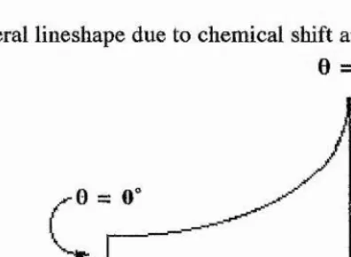
The shielding that the central carbon experiences varies with 0. Therefore, a wide chemical shift range is observed (figure 1.6). Since there are more perpendicular arrangements (9 = 90°) than parallel (0 = 0°) this gives a more intense peak.
Figure 1.6: General lineshape due to chemical shift anisotropy.
cluenûcal sMft
These effects, dipolar coupling and chemical shift anisotropy, are not observable in solution NMR as the rapid molecular tumbling averages the dipolar vectors and the anisotropy to zero. This decouples the magnetic nuclei by the rapid changing of their orientations and leads to a single isotropic chemical shift.
1,2.3. High Resolution Solid-state Spectra
As we have seen above, in the solid-state, chemical shift anisotropy and direct dipolar coupling lead to line broadening in the spectrum and, thus, must be removed if we are to obtain high resolution spectra.
Each of these effects contain the term (3cos^0 - 1). Where 0 is the angle
determining the orientation of the molecule with respect to Bp. If the nuclei can be
“fooled” into believing that (3cos^0 - 1) equals zero, then these interactions become
[image:30.612.184.382.167.312.2]For 3cos20 - 1 = 0
Scos^G = 1
cos^G = 1/V3 G = 54.74°
This is the Magic Angle.
The magic angle (G^) turns out to be the angle between the opposite vertices of
a cube. If the nuclei are spun about the magic angle the average interaction is along Gm-
Therefore, anisotropic interactions are greatly reduced (figure 1.7).
Figure 1.7: The Magic Angle.
Spinning the sample about 0m averages the direction of all the Na/Nb interactions.
The average of the vector AB is the magic angle.
The sample is either machined into the shape of a rotor or packed into a ceramic rotor and the rotor is spun by an air turbine around the axis of the magic angle. In addition, double irradiation at the proton frequency decouples the protons firom the This is the same as the scalar decoupling discussed earlier but, it requires much more power to do.
1.2.4. Cross Polarisation Sequence
Figure 1.8: The Cross Polarisation Pulse Sequence.
step 2 step 3
By using cross polarisation it is possible to obtain spectra without using a
long relaxation delay. In addition, cross polarisation enhances the signal intensity for
13C. Basically it involves the enhancement of the magnetisation of the rare spins (^^C)
from that of the abundant spins (^H). In the first step (figure 1.8) the spins are
flipped over onto the y'-axis by a 90° pulse along the x’-axis and then spin-locked by a
RP pulse along the y’-axis. The spins are kept locked along the y’-axis for a time
period t. In this time the spin lock field is applied. Thus both sets of spins are
spin-locked onto the y’-axis. By choosing the correct frequency of spin-locking fields
Hiji and the net carbon magnetisation may be enhanced by the proton reservoir
(step 2). This is the contact period. The magnitudes of the two fields are chosen such that the Hartmann-Hahn condition (Eq. 1.7) is met.
= Y|3cH i3c (Eq. 1.7)
Since ~ 4/1, the spin locking field must be four times to
precess about the y’-axis with the same frequency. Therefore, the energy required for spin flips between the two spin energy levels is the same for both nuclei and thus the nuclei will accumulate magnetisation from the proton reservoir. The loss of proton
magnetisation during this process is negligible. After the magnetisation has built
up during this contact period, the spin locking field is switched off and the carbon
FID recorded (step 3). The proton field remains on to decouple the proton-carbon dipolar interactions. There is then a time delay in which the protons and carbons are allowed to relax towards their equilibrium values (step 4). In contrast to the simple pulse-FT experiment, the carbon magnetisation for the FID does not depend on the relaxation of the carbon spins in the delay period, but arises entirely from the contact with the proton spins. This means that the intensity of the carbon spectrum effectively depends on the relaxation of the proton spin system. This is much shorter than the relaxation of the carbon spin system and thus the recycle time for effective accumulation
is much shorter than for a conventional pulse-FT experiment.. A further advantage
of these spectra is that carbons which are difficult to observe in solution, e.g. carbonyls and quaternary carbons, have intensities comparable to other carbons in the system.
In conclusion the total CP/MAS experiment involves the use of
Cross-polarisation techniques to increase the S/N and to bypass the Ti relaxation processes of the dilute nuclei being observed.
High power proton decoupling during acquisition to remove the dipolar and scalar interactions.
Continuous magic-angle sample spinning to remove the chemical shift anisotropy and further reduce dipolar interactions.
1.2.5. Spectral Editing in the Solid-State
of 13c spectra in solution. This is because the solid-state interactions being removed by decoupling are dipolar in nature and must be completely removed during acquisition. The dipolar interaction between two spins depends dramatically on the internuclear distance and there will thus be a very large difference in the dipolar broadenings of carbon atoms with one or more hydrogens attached compared to those of carbons with no attached hydrogens. It is therefore possible to distinguish between these two types of carbon atoms using a modification of the CP pulse sequence. This is known as
dipolar dephasing.
1.2.5.1. Dipolar Dephasing
Figure 1.9: The Non-quaternary Suppression (NQS) Pulse Sequence. Pube
H
I
lock^ decouple ^
10
^ contact ^ FID
variable delay of typically 50 |jl3
Effectively, this technique is used to suppress resonances due to CH2 and CH
(non-quaternary) carbons leaving only CH3 and quaternary C peaks. The pulse
dephase them. After a short period (typically 50 ps) the decoupling field is reapplied to decouple the dipolar interactions during acquisition of the carbon FID. The spectmm now contains only quaternary and methyl carbons (for methyl carbons, the dominant mechanism for relaxation is by spin rotation).
Thus: Quaternary carbons aie least affected,
CH3 is next least affected,
CH and CH2 can be edited out if a suitable delay is applied.
1.3. Two-Dimensional NMR Spectroscopy ^ Figure 1.10: The 2D Pulse Sequence.
Mo
/
• M l MisinZTWtiM, =
90° 90°
M]Cos27Cvt]
Acquisition (t])
A sample with only one resonance line in its' spectrum, such a chloroform,
will have a chemical shift, v. After a 90° pulse the spin vector, M%, processes in the x’- y’ plane. In figure 1.10, Mi processes in the x’-y’ plane at v cycles per second for a time t%. At the end of this interval, t%, a second 90° pulse is applied along the x’-axis and the NMR signal is measured as a normal FID. The result of this is that the vector has processed through an angle of 27Wti during the interval, so, if its length is M, then the component along the y’-axis is Mcos27rvti and that along the x’-axis is Msin27cvti.
The value of M is related to the initial magnetisation Mq by
M = M (E q. 1.8)
magnetisation left in the x’-y’ plane is Msin2jcvti and determines the size of the NMR signal. The spectrum obtained is perfectly normal apart from a change in amplitude.
If a series of experiments with different values of ti, e.g. values from 0 to a few seconds, are performed and the data from each experiment transformed into a spectrum, then a series of peaks is produced with size varying with ti. The height of the peaks would oscillate sinusoidally with frequency v as the transverse magnetisation at the end of ti is given by Msin27tvti.
By taking the point from each experiment that corresponds to the top of the peak and plotting these points as a function of ti, a graph of the signal amplitude is obtained,
which is oscillating with frequency v and decaying exponentially with time constant T2.
The graph is exactly like an FID. A Fourier transform of the graph gives a frequency spectrum with one line, exactly the same as the normal FIDs that made up the spectrum. However, it is normal practise to perform Fourier transforms on every column of points taken from the complete set of FIDs. The two-dimensional Fourier transform converts the data into a two dimensional frequency spectrum which is a function of Vi
and V2. V2 is the chemical shift of the peak as is Vi. Thus we get a square spectrum
with both axes representing chemical shifts and a peak appearing in the frequency domain at (v,v), i.e. on the diagonal.
This experiment contains no more information than a simple one-dimensional spectrum but contains the basic principles of two-dimensional NMR in which a signal,
modulated as a function of ti, is detected as a function of t2. All two-dimensional
experiments are performed in this way.
1.3.1. Two Dimensional Exchange Spectroscopy
frequency labelled z-axis component is involved is chemical exchange with another nucleus.
If we wait a while after the second pulse, using the pulse sequence:
-2 ~ ‘i ~ 2 - 2 “ ‘2
then in the presence of exchange a nucleus whose z magnetisation was modulated by one chemical shift during ti may have the opportunity to migrate to another site during
Xm» the mixing time. Thus it has a different chemical shift during t2 and the resulting
spectrum will have cross-peaks between the shifts of the exchange sites.
Xm has to be selected so that the maximum amount of exchange takes place before the final pulse samples the z magnetisation. This requires knowledge of the Ti ’s of the nuclei involved and of the rate of exchange. However, the purpose of the experiment is to determine these parameters. Chemical exchange can be occurring at any rate but must be in the slow exchange regime to be detected by this method. Therefore an upper limit can be imposed on the rate according to the shift differences involved. For two-site exchange between nuclei with equal populations and shift difference Av the coalescence rate kc is
k g = ^ ...(Eq. 1.9)
The exchange rate must be less than k^. At the other extreme, k must not be much less
than 1/T1 or the z magnetisation will disappear before it has a chance to migrate. The
range of useful k values lies between these limits and guesswork must be applied for the value of Xm to be used.
1.4. Dynamic NMR Spectroscopy
simplification of NMR spectra discussed earlier. However, there are a great number of more subtle intramolecular motions and these can, in certain cases, produce effects which are observable in the NMR spectrum.
Much work has been done to determine rates of motion in the gas and, especially, the solution phases. However, until recently, no-one even considered the possibility of molecular motions, aside from vibrations, taking place in the solid as the restricting nature of the crystal lattice should make such processes very difficult indeed. However, the relatively few studies performed in the solid-state show this not to be the case and many molecules in the solid-state are now known to be motionally labile. It is with this in mind that a study of molecules likely to exhibit motion in the solid-state should be undertaken to address the present imbalance.
In general, when the rate of a molecular motion equals or nears the rate of an NMR process then the motion may interact with that process to produce an observable effect in the NMR spectrum. This is the basis of dynamic NMR spectroscopy. Since the rate of the motion is invariably linked to the temperature of the sample, then by measuring or simply observing the change in the spectrum with temperature, it may be possible to calculate the rate and hence, the parameters for the motion, i.e. Ea, AG$, AH$, and AS$.
There are many processes in operation in the acquisition of a spectrum and the frequencies of these processes cover an enormous range. The processes used to measure rates in this thesis are outlined below and are arranged in increasing frequency, beginning with the slowest.
1.4.1. Two Dimensional Exchange Spectroscopy
The details of this experiment are detailed above. This method is appropriate
for measurements of rates comparable to spin lattice relaxation rates from 10 to 10 3
s"l.
1.4.2. Chemical Shift Difference
When the rate of motion is less than the chemical shift difference then the shifts of the nuclei in each position are shown in the spectra. As the rate increases towards the chemical shift difference then the corresponding shifts merge together until the rate of motion is greater than the chemical shift difference and an average signal is observed at the mean distance between the peaks. This convergence of shifts is known as coalescence and the temperature at which this occurs is important in the determination of the rate of the motion. The rate of exchange at coalescence is determined using equation 1.9 and the free energy of activation can be calculated using the Eyring equation thus
A G / =19.1Tc(10.32 + logTc~logkc) (E q. 1.10)
This method of measurement is sensitive to motions in the region 10^ to 10^ s'l.
1.4.3. Maximum Dipolar Broadening
Maximum dipolar broadening occurs when the frequency of the incoherent molecular motion is the same as that of the coherent decoupler^^. This reduces the decoupling efficiency and so broad lines result. Its maximum is when k = coi.
Since coi 50-100 kHz, this permits a single rate in this range to be measured.
1.4.4. T ip Relaxation
When the rate of motion nears the frequency of the l^C spin lock field, typically 50-100 kHz, it modulates the relaxation in the rotating frame making it more efficient. By measuring the rate of relaxation, i.e. the time constant Tip, the rate of motion can be calculated39. Measurement of rates in the region of 1(H to 10^ S“^ can be made.
Using a combination of some or all of these techniques, rates of rotation can be
1.5. What is a Conformation?
The term conformation was originally used to denote any one of the infinite number of arrangements of the atoms in space that result from rotation about single bonds. An example of this is the rotation about the C-C bond in ethane. However, this view is too simplistic. The arrangement of the atoms with respect to each other in a molecule of cyclohexane, is not fixed^. The individual arrangements are not simply related by bond rotation but are still defined as being conformations of the molecule. For the conformations to interchange, the molecule must not only undergo bond rotations but also bond angle deformations. Therefore, the classical description of a conformation must be expanded to accommodate this. In general, a conformations can be interchanged by rotation about a single bond with any resultant small distortion in bond lengths and angles or by inversion at a three coordinate centre in the molecule.
1.6. Factors Influencing Conformation
Up until the mid 1930’s rotation about single bonds was thought to be free in nature. However, theoretical calculations of thermodynamic parameters were in poor agreement with experimental results. Good agreement was not reached until baiiiers to bond rotations were incorporated into the calculations.^'^ In ethane, this barrier is the result of the hydrogens becoming alternately eclipsed and staggered as the methyls rotate with respect to each other. The energy differences between the staggered and eclipsed conformations are due to interactions in the electron clouds in the C-H bondsl^.
In the pursuit of conformational information, chemists turn to the classical approach of molecular mechanics. In this approach the conformational energy of the molecule is broken down into the following components;
Torsional forces
Bond angle deformation Electrostatic interaction Solvent effects
Hydrogen bonding
The quantitative interactions are described below.
1,6.1. Torsional Forces
The general form of the potential function for rotation about a single bond is:
E((|)) =-y Eg(l + cos H(j))
" (Eq. 1.11)
E((j)) is the energy when there has been a rotation of (j) from the eclipsed position. En terms are energies associated with each n-fold component of the total function.
The simplest example of rotation about a single C-C bond is that of ethane in which only a three-fold barrier is important^^; Figure 1.11:
E($) = 1 E3(1+cos3$) ^ 12.24 kJmoH
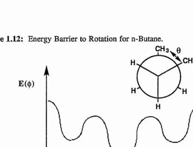
For n-butane there are two components; a one-fold eclipsing of methyls and a
three-fold eclipsing of any group; Figure 1.12.
E(({)) = ^E i (l+cos{})) + (l+cos3(|))
Figure 1.11: The Potential Barrier to the Rotation of Ethane.
120 ISO 240
0 60
Dihedral Angle,0 (Degrees)
Figure 1.12: Energy Barrier to Rotation for n-Butane.
0 60 120 ISO 240 300 360
Dihedral angle, 0 (degrees)
1.6.2. Non-bonded Interactions
[image:42.612.116.433.339.581.2]E(r) = Ae-Br . Cr'6... (Eq. 1.12)
where E(r) is the interaction energy, r is the distance separating the interacting atoms and A, B and C are constants for the atom pair concerned. The distance at which repulsive and attractive forces between two atoms are equal, i.e. E(r) = 0, is known as the van der Waals distance.
1.6.3. Bond Stretching
Deformation of conformation due to bond stretching is generally small. The expression concerned is an harmonic function:
E(l) = A (l-lo)2... (Eq. 1.12)
where 1 is bond length in pm and 1q is the equilibrium bond length. The typical function
for a C-C stretch is thus^l,
E(l) = 0.3168(1-152.0)2 (Eq. 1.13)
1.6.4. Bond Angle Deformation
Bond angle deformations have the following functionl3-l4.
E(0) = Ke(0 - x)2... (Eq. 1.14)
where Ke is the force constant, 0 the new angle and x the original undeformed angle,
deformation in the C-C-C bond angle of 4 \ It is easy to see that most of the strain in a molecule will be relieved by deformation of the bond angles.
By careful consideration of all these interactions a picture can be built up of the likely conformation adopted by a specific molecule when free in solution or in the gas phase. Lattice packing forces in solids can lead to molecules crystallising in conformations other than those preferred in solution.
1.7. Conformational Analysis Before NMR
Many measurable physical properties can be used to determine the conformation of a molecule. These properties include dipole moment, electron and X-ray diffraction and spectral properties. Examples of their use in the elucidation of conformation are thus:
1.7.1. Dipole Moment
The anti and gauche forms of 1,2-dibromoethane differ in dipole moment. In
the anti form the C-Br bond dipoles are antiparallel and the dipole moment is zero. The
actual dipole moment of 1,2-dibromoethane^^ is approximately 1 debye unit and thus
the molecule doesn’t exist solely in the anti form. The dipole moment also varies with
temperature and so the molecule cannot exist solely in the gauche form either.
Therefore, either the anti and gauche forms are in equilibrium with each other and this
varies with temperature or the molecule exists in either foim and librates about the C-C bond without passing into the other form.
1.7.2. X-ray and Electron Diffraction
If the molecule under investigation contains relatively heavy atoms then the position of these atoms can be determined using electron diffraction and thus the
conformation will become known. 1,2-dihaloethanes^^ aie known to exist in the anti
Measurements on n - b u t a n ehave indicated that 60±15% of the molecules exist in the
anti conformation at 14"C
X-ray diffraction has been used to determine the conformation of molecules in the solid-state. The X-ray pattern of 1,2-dichloroethane^^ shows that it crystallises
exclusively in the anti form. It is possible, however, for a molecule to crystallise in
more than one conformation. Indeed, 1,1,2,2-tetrabromoethane^^ crystallises in a mixture of the two conformations.
1.7.3. Spectroscopy
This is perhaps the most important method of conformational analysis, especially NMR. Before its advent, many conformational analyses had been performed using infrared, Raman and microwave spectroscopy.
Infrared depends upon vibrations leading to a change in molecular dipole moment. Raman depends upon vibration leading to a change in molecular polaiisabüity.
17.3.1. Infrared and Raman Spectra
The maximum number of vibrations and hence infrared and Raman lines, in a non-linear molecule of N atoms is 3N-6. A molecule like 1,2-dibromoethane shows the allowed number of lines in the solid-state spectrum but additional lines are present in the liquid and gas phases. The solid-state spectrum shows that the molecule has a
centre of symmetry and thus must crystallise in the anti conformer. On liquefaction,
some molecules transform to the gauche form.20 In principle, the position of the
equilibrium of the anti and gauche forms of 1,2-dibromoethane can be calculated from
the intensity of the spectral lines using a variation of Beer’s Law^^:
' - . ( S )
where, the superscript t and g refer to trans and gauche respectively, N is the number of molecules per millilitre, E is the molecular extinction coefficient and Iq and I are the intensities of the incident and transmitted radiation.
1.7.3 2. Microwave Spectroscopy
Microwave spectra have been used to arrive at estimates of the energy barriers to eclipsed conformations. The height of the barrier can be found from the frequency
1.8. The Principle of Least Distress
Conformational processes in the gas and solution phases are relatively unhindered by neighbouring molecules. However, in the solid-state, the crystal lattice makes it more difficult for conformational processes to occur and consequently their energies of activation are expected to be higher. In the crystal lattice, the majority of atoms have low amplitude motion and act as a reference frame against which a smaller conformationaUy mobüe group can move. Conformational processes are more likely to occur, and thus be observed by NMR, where there is a small volume change involved during the motion. This idea is termed the principle of least distresses. When the conformational process involves the rotation of a group about a single bond, then the more symmetrical the group is, the more easily it will rotate. This principle is demonstrated in figure 1.13.
Figure 1.13: A Rotating Group with Ligands of Differing Size Neighbouring
Molecule Profile
120"
rotation
Experimental
2.1 Symbols and Abbreviations
mol moles
h, min hours, minutes
NMR nuclear magnetic resonance
ppm parts per million
Hz hertz
J spin-spin coupling constant in Hz
s, d, t, q, m singlet, doublet, triplet, quartet, multiplet
ABq AB quartet
ABX ABX multiplet
m.p. melting point
b.p. boiling point
2.2 Instrumentation
2.2.1 Solution NMR Spectroscopy
All iH and solution spectra were obtained on either a Bruker MSL500
spectrometer operating at 500.130 and 125.758 MHz respectively or on a Varian Gemini 200 operating at 200.052 and 50.303 MHz respectively. The quaternary ammonium and phosphonium salts were referenced to methanol (lH-3.5 ppm and
13C-49.3 ppm) in D2O and the amines and borane complex to TMS (^H-0 ppm and
l^C-O ppm) in CDCI3.
2.2.2 Elemental Analysis
2.2.3 Melting points
All melting points were earned out on an Electi‘othermal melting point machine. The temperatures are uncorrected.
2.3 Solid-State Spectra
All solid-state NMR spectra were obtained on a Bruker MSL500 spectrometer
in either high resolution or high power mode. Solid-state spectra were obtained at
125.758 MHz in the CP/MAS mode using 4 mm o.d. rotors spinning typically at 6-8
kHz. All solid-state spectra including Tip determinations were obtained by the cross polarisation pulse sequence. However, in the case of compound 4 the pulse sequence
incorporates a 50 |LLS dipolar dephasing delay, sufficient to dephase any non-mobile
carbons dkectly bonded to one or two hydrogens. A cross polarisation contact time of
1 ms was used throughout.
Chemical shifts were referenced relative to the CH2 group in adamantane at
38.56 ppm determined on a separate sample.
The 2D CPEXSY spectra were obtained using a standard pulse sequence
including a 1 ms contact time and a mixing time ca. 100-200 ms.
The l^C spin locking frequency during the Hartmann-Hahn condition was determined using single carbon pulses and high power ^H decoupling on adamantane and was found to be in the region 60-90 kHz. The same radio frequency power was used for the spin lock period in the Tip determinations.
All spinning side bands shown in the spectra are marked thus:
2.4 Calibration of the Variable Temperature Unit [BYT 1000]
The unit was calibrated using the 4 mm MAS probe. Variable temperature
spectra were run on compounds with known phase changes^^. A few samples were
thesis, thus minimising the effects of heating arising from sample spinning and high power decouplings^.
Sample Phase ChangeTemperature. VT UnitSetting Observations
d-camphor 374 405 CPCYCL but HPDECLoss of efficiency of
works OK.
d,l-camphor 350 380 Doubling of several lines.
pivalic acid 280 271 At high T, t-butyl methylis a singlet. At low T it
is a doublet.
d-camphor 244.5 223 Change in all signals.
adamantane 209 186 replace 38.56 ppm.Extra broad signals
2.5 Line shape Analysis
Figure 2.1: Compounds Prepared for Study
/ " V - C H , ,C H , / ^ V - C H j ,CH3 ,C H ,
\ = / H—N— 0— H \ = / H— N - C - C H j \ = = / H - N - C - C H 2 C H 3
H 6(a) C", H 6(b) CH, » 6(c)CHs
/ ~ \ - C H 3^ ,C H , / ~ y - C H 3^ ,C H , / ~ y _ c H 3 ^ ,C H ,
\ --/ H — N—C—H \ = / H—N—C—CH
3\sr=/ H—N—C—CH
2CH
3ch: CH: c h:
r y
oj
,c h 3 r yfy
/ CH3-N— C""H X ssss/ CH3~N“~ C ~ CH3 \ = / CHs"N"“ C” CH2CH3
CH^ 'CH3 CH3 CHg CH3 CH3
8(a) 8(b) 8(c)
O- f\ f\
.N— C-H
(y
.N—C
7CH
3'n—C-f \ Br- Be-
Br-H—.N—' c—H
H—.N""
0~CH
3H—N—c-a
CH
2CH
3CHg
CH
310(a) y V 10(b)
CHg CH3
10(c)
/~V-CHa
+,CHa/ ^ V ” CHa
+,CH,CHa
.,CH,—C— Nr-H
H yC
CH
3X—y H yC
CHgCHg
h'
CH
3H
CH
3H
CH
311(a) 11(b) 11(c)
/ ~ ^ C H a + ,C H , / ~ V - C H a / " \ - C H a . ,C H ,
\ = / H—C— N;-H \ = / H—C—N—CHa \ = / H — C— N— CHgCHg
CH3 OHj CHj CH3 CH3 CH3
12(a) 12(b) 12(c)
Br"
f\
Br-y
Br-'* « & X ''C H a +,CH3 > « S ^ C H a U s , y ^ CH
H —C—N—H
H —C—N— CH
3H—
r v s a
r v s a
l y s
\s=»^ l.lfal 13(a) 13(b) 13fh) \s=='Ns==' 13(c)
/~ V - C H a ,,CH3 ^ " ^ C H a .^CHa
\ = = / H - C —P^-C H ; \ = / H—
H^" CH3 CH3 CH3
2.6 Synthesis
Elemental Analyses of compounds prepaied are given in Table 2.2.
A Preparation of Compounds 6(a), (b) and (c).
A1 Prepaiation of N-Benzvl-Alkvlammonium Bromide
Benzyl bromide [3.42g, 0.02 mol] was added to a large excess of amine [50ml] slowly with cooling, and the resultant precipitate filtered off and recrystallised [ethanol/ether].
A l.l Preparation of Compound 6(a)
The method of A1 was followed using /-propylamine to afford compound 6(a)
(4.38g, 95%) as white crystals, m.p. 215-216 °C; NMR (D2O) 1.5 (6H, d, J 6.5,
2 CH3), 3.7 (IH, m, J 6.5, N-CH), 4.4 (2H, s, CH2) and 7.6 (5H, m, Ph); I3c
NMR (D2O) 18.6 (2 CH3), 48.6 (CH2), 60.0 (N-CH), 129.6 (C-2% 6'), 129.8 (C-3\
5'), 130.0 (C-4’) and 131.5 (C-1’).
A1.2 Preparation of Compound 6Cbl
The method of A1 was followed using f-butylamine to afford compound 6(b)
(3.77g, 78%) as white crystals, m.p. 236-238 "C; NMR (D2O) 1.6 (9H, s, 3
CH3), 4.3 (2H, s, CH2) and 7.6 (5H, m, Ph); l^C NMR (D2O) 25.3 (3 CH3), 45.8
(CH2), 58.3 (4ry C), 129.6 (C-2',6'), 129.7 (C-4'), 129.9 (C-3',5') and 131.8 (C-1')
A1.3 Preparation of Compound 6Cc)
The method of A1 was followed using f-amylamine to afford compound 6(c)
(4.28g, 83%), as white crystals, m.p. 207-208 “C; iH NMR (D2O), 1.2 (3H, I, J 7.5,
Et-C H3), 1.6 (6H, s, 2 CH3), 1.9 (2H, q, J 7.5, CH2), 4.4 (2H, s, CH2) and 7.6
(5H, s, Ph); 13c NMR (D2O) 7.5 (Et-CH3), 22.6 (2 CH3), 30.9 (Et-CHz), 45.5 (N-
CH2), 61.4 (4ry C), 129.6 (C-2', 6'), 129.8 (C-4'), 130.0 (C-3', 5') and 131.8 (C-
B Preparation of Compounds 7(a), (b) and (c).
Methods B l-3 & 6 were used in the preparation of compounds 7(b) and (c).
However, this method was not effective for the preparation of compound 7(a) and methods B4-6 were employed instead.
B1 Benzovlation of the Amine
The amine [0.2 mol] was dissolved in NaOH solution [240 ml, 5%] and to this was added benzoyl chloride [30g, 0.21 mol]. The mixture was stirred vigorously for two hours and the resultant precipitate filtered off, recrystallised (ethanol), and dried to give white crystals.
B l.l Preparation of r-Butvl Benzamide.
The general method B1 was followed using f-butylamine to afford
t-butylbenzamide (20.76g, 59%) as a white crystalline solid, m.p. 132-133 °C.[Lit. m.p. = 131-2 “C]25a
B1.2 Preparation of f-Amvl Benzamide.
The general method B 1 was followed using f-amylamine to afford
t-amylbenzamide (26. Ig, 68%) as a white crystalline solid, m.p. 92-94 “C.[Lit. m.p. =
112-3 “C]25a
B2 Alkvlation of the Amide
NaH [4.4g, 0.11 mol (60% in oil)] was dissolved in dry THF [100ml] and to
this was added the amide [0.1 mol] and the mixture heated under reflux for 1 hour.
B2.1 Méthylation of the r-Butvl Amide.
The general method B2 was followed using the r-butyl amide and methyl iodide to afford the methylated f-butyl amide (13.5g, 71%) as a low melting solid.
B2.2 Méthylation of the r-Amvl Amide
The general method B2 was followed using the f-amyl amide and methyl iodide
to afford the methylated /-amyl amide (14.8g, 68%) as a low meting solid.
B3 Reduction of the Amide
The amide [0.04 mol] was dissolyed in dry THF [20ml] and added dropwise to
a solution of LiAlH4 [1.48g, 0.044 mol] in dry THF [50ml]. The mixture was heated
under reflux for 1 hour after which NaOH [1.48g, 0.04 mol] in water [1ml] was added
to giye a white precipitate. The solution was decanted, dried [K2CO3], and the solyent
remoyed.
B3.1 Preparation of N-Benzyl-N-methyl-/-butylamine.
The general method B3 was followed using the /-butylamide to afford the
benzylmethyl amine (6.7 8g, 96%) as a clear liquid.
B3.2 Preparation of AT-Benzyl-A^-methyl-/-amylamine.
The general method B3 was followed using the /-amylamide to afford the benzylmethyl amine (6.99g, 91%) as a clear liquid.
B4 Benzylation of the Amine
The amine [11.8g, 0.2 mol] was added to NaOH [8g, 0.2 mol] in water
B5 Mono-Methvlation of the Amine. /The Eschweiller Clai'k Reaction)
The amine [2.98g, 0.02 mol] was added to 40% aqueous formaldehyde [1.5g, 0.02 mol] in water [12,5ml] with cooling in ice/water. To this was added 98% foiTnic
acid [0.94g, 0.02 mol] and the solution heated under reflux for 6 hours. After this
time, NaOH pellets [0.8g, 0.02 mol] were added and the resultant mixture extracted
with ether, dried[K2C03], and the solvent removed to leave a yellow hquid.
B5.1 Preparation of A^-Benzvl-iV-methvl-/-propvlamine.
The general method B5 was followed using N-benzyl-/-propylamine to afford N-benzyl-/V-methyl-/-propylamine (2.56g, 79%) as a yellow liquid.
B6 Hvdrobromination of the Amine
The amine [0.01 mol] was dissolved in ethanol [20ml] and to this was added 48% hydrobromic acid [L69g, 0.01 mol]. The solvent was removed leaving a white solid which was recrystallised [ethanol/ether].
B6.1 Preparation of compound 7(a")
The method of B6 was followed using /-propylamine to afford compound 7(a)
(2.31g, 95%) as white crystals, m.p. 132-134 “C; ^H NMR (D2O) 1.5 (6H, d, 7 7 ,2
CHg), 2.8 (3H, s, N-CH3), 3.8 (IH, m, 7 7, CH), 4.4 and 4.6 (2H, ABq, 7 12 N-
CH2) and 7.6 (5H, m, Ph); NMR (D2O) 16.2 (2 CHg), 35.4 (N-CHg), 56.9 (N-
CH2), 57.6 (N-CH), 129.6 (C-2%6'), 130.3 (C-4'), 130.8 (C-1') and 131.0 (C-
3%5').
B6.2 Preparation of Compound 7(b')
The method B6 was followed using /-butylamine to afford compound 7(b)
(2.30g, 89%) as white crystals, m.p. 180-181 "C; ^H NMR (D2O) 1.7 (9H, s, 3
Ph); 13c NMR (DoO) 24.3 (3 CHg), 34.0 (N-CHg), 55.1 (N-CH2), 64.7 (4ry C),
129.6 (C-2’,6’), 130.2 (C-4’), 130.4 (C-1’) and 131.2 (C-3’,5’).
B6.3 Preparation of Compound 7(c)
The method B6 was followed using /-amyl amine to afford compound 7(c)
(2.27g, 84%) as white crystals, m.p. 156-157 "C; ^H NMR (D2O) 1.2 (3H, t, 7 7.5,
Et-CHg), 1.6 (6H, s, 2 CHg), 2.1 (2H, q, Et~CH2), 2.8 (3H, s, N-CHg), 4.1 and 4.8
(2H, ABq, 7 12, N-CH2) and 7.6 (5H, m, Ph); l^C NMR (D2O) 7.8 (Et-CHg), 21.2
(2 CHg), 29.5 (Et-CH2), 34.0 (N-CHg), 54.9 (N-CH2), 68.3 (4^7 C), 129.6 (C-
2’,6’), 130.2 (C-4’,1’) and 131.3 (C-3’,5’).
C Preparation of Compounds 8(a), (b) and (c)
C l Dimethvlation of the Amine (The Eschweiller Clark Reaction)
The amine [0.25 mol] was added to 40% aqueous formaldehyde [35g, 0.5 mol] in water [12.5ml] with cooling in ice/water. To this was added 98% formic acid
[23.5g, 0.5 mol] and the solution heated under reflux for 6 hours. After this time,
NaOH pellets [lOg, 0.25 mol] were added and the resultant organic layer separated,
dried[K2C03], and distilled.
C l.l Preparation of T/.A'-Dimethvl-z-propvlamine.
The general method Cl was followed using /-propylamine to afford dimethyl-/- propylamine (13.7g, 63%) as a colourless oil.
C1.2 Preparation of 7/.A/-Dimethvl-/-butvlamine.
The general method Cl was followed using /-butyl amine to afford dimethyl-/- butylamine (14.4g, 57%) as a colourless oil, b.p. 90-91 “C.
C1.3 Preparation of /V. A-Dimethvl-/-amvlamine.
C2 Benzylation of the amine
The amine [0.04 mol] was added to a solution of benzyl bromide [6.84g, 0.04 mol] in ethanol [20ml] and the solution heated under reflux for 1 hour. The solyent was remoyed leaying a white solid which was recrystallised from ethanol/ether.
C2.1 Preparation of Compound 8(a^
The method C2 was followed using /-propylamine to afford compound 8(a) (3.09g, 46%) as a white crystalline solid, m.p. 205-206 'C; % NMR (DgO) 1.6 (6H, d, J 6.5, 2 CHg), 3.1 (6H, s, N-CHg), 3.8 (IH, m, J 6.5, CH), 4.6 (2H, s, N-CH2), and 7.7 (5H, m, Ph); 13c NMR (D2O) 16.3 (2 CHg), 47.0 (2 N-CHg), 65.4
(N-CH2), 66.4 (N-CH), 127.7 4’), 129.4 2’,6’), 130.9 1’) and 133.2
(C-3’,5’).
Crystal data: Ci2H2oNBr, Mj- = 258.2, orthorhombic, Pcab, a = 9.7610(2)Â, b
= 29.896(1)Â, c = 10.0389(2)A, V = 2537.6Â, Z = 8, Dc = 1.17 g cm'3. The
structure was solyed from X-ray powder diffraction data collected on a Stoe STADI/P
transmission system, X - 1.54056Â (CuK^i). Data was collected oyer the range
5“<20<85“ in 0.02^ steps, the entire run lasting about 15 hours. Data was indexed on
the basis of the first 20 obseryable lines using the program TREOR (M20 = 21.6). The
pattern decomposition option of the Rietyeld program GSAS was used to extract the first 121 integrated intensities from the powder pattern. These were used as input to the direct methods program SIR (12), from which the Br atom was located. The remaining atoms were found yia successiye difference Fourier / least squares cycles applied to Rietyeld refinement of the whole diffraction profile. In the final stages of refinement, chemical constraints were added (C-C (ring) = 140(1)Â, C-C-C (ring) = 120", C-C
(exo) = 155(1)Â, C-N = 157(1)Â). Final agreement indices were Rwp = 8.4%, =
C2.2 Preparation of Compound 8[b)
The method C2 was followed using /-butylamine to afford compound 8(b)
(3.9g, 36%) as a white crystalline solid, m.p. 196-197 "C; NMR (D2O) 1.7 (9H,
s, 3 CHg), 3.0 (6H, s, 2 N-CHg), 4.6 (2H, s, CH2) and 7.7 (5H, m, Ph); l^C NMR
(D2O) 21.5 (3 CHg), 42.2 (2 N-CHg), 59.8 (CH2), 71.5 (4>T C), 126.0 (C-4’), 127.1
(C-3’, 5’), 131.6 (C-2’, 6’) and 128.6 (C-1’).
C2.3 Preparation of Compound 8(c]
The method C2 was followed using /-amylamine to afford compound 8(c)
(3.48g, 32%) as a white crystalline solid, m.p. 174-175 "C; ^H NMR (D2O) 1.3 (3H,
t, J 7, CHg), 1.8 (6H, s, 2 CHg), 2.2 (2H, q, J 7, CH2), 3.0 (6H, s, 2 N-CHg), 4.6
(2H, s, N-CH2) and 7.7 (5H, m, Ph); 13c NMR (D2O) 9.7 (Et-CHg), 19.8 (2 CHg),
27.9 (Et-CH2), 44.4 (2 N-CHg), 62.1 (N-CH2), 78.5 (4^7 C), 128.3 (C-1’), 129.3
(C-2’, 6’), 130.8 (C-4’), 133.8 (C-3’, 5’).
D Preparation of Compounds 9(a), (b) and (c) D l l Preparation of N-Benzovl-/-butvlamine.
The general method B1 was followed using /-butylamine to afford N-Benzoyl-f- butylamine (20.76g, 59%) as white crystals, m.p. 132-133 "C.
D1.2 Preparation of N-Benzovl-/-amvlamine.
The general method B1 was followed using /-amylamine to afford N-Benzoyl-/-
amylamine (26. Ig, 68%) as white crystals, m.p. 92-94 "C.
D2.1 Alkvlation of the /-Butvl Amide.
D2.2 Alkvlation of the /-Amvl Amide.
The general method B2 was followed using the /-amyl amide and benzyl bromide to afford the benzyl amide (4.45g, 40%) as white crystals, m.p. 69-72 °C
D3.1 Reduction of the /-Butvl Amide to Afford Compound 9tbl
The general method B3 was followed using the /-butyl benzyl amide (0.02 mole equivalent) to afford the dibenzyl amine, 9(b), (2.63g, 52%) as white crystals, m.p.
66-68 "C; % NMR (CDCI3) 1.2 (9H, s, 3 CH3), 3.8 (4H, s, 2 CH2) and 7.3 (lOH,
m, Ph); 13c NMR (CDCI3) 27.5 (3 CH3), 54.3 (2 N-CH2), 55.6 (40- C), 126.0 (C-
4’). 127.0 (C-2’, 3’, 5’, 6’) and 142.8 (C-1’).
D3.2 Reduction of the /-Amvl Amide to Afford Compound 9(c).
The general method B3 was followed using the /-amyl benzyl amide (0.02 mole equivalent) to afford the dibenzyl amine, 9(c), (3.45g, 65%) as white crystals, m.p.
41-42 “C; IH NMR (CDClg) 1.2 (3H, t, 7 7.5, Et-CHg), 1.8 (6H, s, 2 CHg), 2.2
(2H, q, 7 7.5, Et-CHi), 3.6 (4H, s, 2 N-CH2), 7.2 (4H, d, 7 7.5, 2, 6), 7.4 (4H, t, 7
7.5, H-3’, 5’) and 7.5 (2H, t, 7 7.5, H-4’); 13c NMR (CDClg) 8.7 (Et-CHg), 24.3 (2
CHg), 32.8 (Et-CHz), 53.8 (2 N-CH2), 58.0 (4^7 C), 126.0 (C-4’), 127.7 (C-3’, 5’),
128.3 (C-2’, 6’) and 142.7 (C-1’).
D4 Preparation of Compound 9Cal
The general method B4 was followed using /-propylamine to afford the dibenzyl amine (6.34g, 27%) as white crystals, m.p. 33-34 “C; ^H NMR (CDClg) 1.0
(6H, d, 7 7, 2 CHg), 2.9 (IH, m, CH), 3.5 (4H, s, 2 N-CH2) and 7.3 (lOH, m, Ph);
13c NMR (CDClg) 18.0 (2 CHg), 48.6 (2 CH2), 53.7 (N-CH), 127.1 (C-4’), 128.6
(C-3’, 5’), 129.0 (C-2’, 6’) and 141.4 (C-1’).
![Table 3.2: Tjp Values (msec) for the r-Butyl Carbons of (4); [coi = 89 kHz]](https://thumb-us.123doks.com/thumbv2/123dok_us/8585173.370294/79.612.72.482.123.519/table-tjp-values-msec-butyl-carbons-coi-khz.webp)

![Table 3.6: Tip Values (msec) for the r-Butyl Carbons of (5); [coi = 63 kHz]](https://thumb-us.123doks.com/thumbv2/123dok_us/8585173.370294/89.612.84.470.75.566/table-tip-values-msec-butyl-carbons-coi-khz.webp)