The depth averaged numerical simulation of laminar thin film flows with capillary waves

The Depth-Averaged Numerical Simulation of

Laminar Thin-Film Flows With Capillary Waves

Bruce Kakimpa

Gas Turbine and Transmissions Research Centre (G2TRC),

University of Nottingham, Nottingham, NG7 2RD, UK e-mail: [email protected]

Herve Morvan

Gas Turbine and Transmissions Research Centre (G2TRC),

University of Nottingham, Nottingham, NG7 2RD, UK e-mail: [email protected]

Stephen Hibberd

Gas Turbine and Transmissions Research Centre (G2TRC),

University of Nottingham, Nottingham, NG7 2RD, UK e-mail: [email protected]

Journal of Engineering for Gas Turbines and Power

Copyright © 2016 by ASME

Paper No: GTP-16-1105

Published online May 24,2016.

doi: 10.1115/1.4033471

The depth-averaged numerical simulation of

laminar thin-film flows with capillary waves

Bruce Kakimpa∗

Research Fellow Gas Turbine and Transmissions

Research Centre (G2TRC) University of Nottingham,

Nottingham, NG7 2RD

Herve Morvan†

Professor

Gas Turbine and Transmissions Research Centre (G2TRC)

University of Nottingham, Nottingham, NG7 2RD

Stephen Hibberd‡

Associate Professor Gas Turbine and Transmissions

Research Centre (G2TRC) University of Nottingham,

Nottingham, NG7 2RD

Thin-film flows encountered in engineering systems such as aeroengine bearing chambers often exhibit capillary waves and occur within a moderate to high Weber number range. Although the depth-averaged simulation of these thin-film flows is computationally efficient relative to traditional VOF methods, numerical challenges remain particularly for so-lutions involving capillary waves and in the higher Weber number, low surface tension range. A depth-averaged ap-proximation of the Navier-Stokes equations has been used to explore the effect of surface tension, grid resolution and in-ertia on thin-film rimming solution accuracy and numerical stability. In shock and pooling solutions where capillary rip-ples are present, solution stability and accuracy are shown to be highly sensitive to surface tension. The common prac-tice in analytical studies of enforcing unphysical low Weber number stability constraints is shown to stabilise the solution by artificially damping capillary oscillations. This approach however although providing stable solutions is shown to ad-versely affect solution accuracy. An alternative grid resolu-tion based stability criteria is demonstrated and used to ob-tain numerically stable shock and pooling solutions without recourse to unphysical surface tension values. This allows for the accurate simulation of thin-film flows with capillary waves within the constrained parameter space correspond-ing to physical material and flow properties. Results ob-tained using the proposed formulation and solution strategy show good agreement with available experimental data from

∗_{Corresponding author. Email: [email protected]}

†_{Email: [email protected]} ‡_{Email: [email protected]}

literature for low Re coating flows and moderate to high Re falling wavy film flows.

1 Introduction

A thin-film may be described as a layer of liquid par-tially bounded by a solid substrate, with a free surface where the liquid is exposed to another fluid - usually a gas [1]. In many applications, the depth of the thin-film is typically or-ders of magnitude smaller than the other lateral dimensions of the liquid expanse. Thin-film flows are central to a num-ber of industrial and process engineering applications such as distillation, absorption, condensation, advanced power ex-traction, photochemistry and surface cooling/heating.

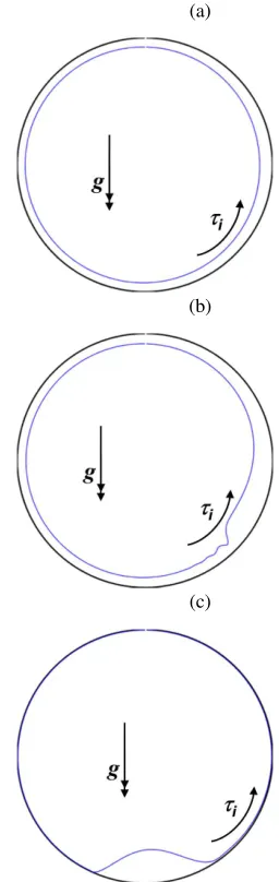
Of particular interest to the present study are the lami-nar shear-driven thin-film rimming flows inside aero-engine bearing chambers where thin liquid films are driven by an inter-facial shear stress in the presence of a gravitational field, surface tension and pressure gradient forces [2], [3, 4]. The problem of a two-dimensional (2D) classical shear driven rimming flow, as shown in Figure 1, has been used to investigate the problem of thin-film flow, assess existing formulations and based on the findings propose a solution strategy. In this idealised model of an aero-engine bearing chamber, a film of liquid is driven over a stationary cylindri-cal outer wall by an interfacial shear stress in the presence of gravity. Film liquid properties used in this study are also described in Table 1, and correspond to a typical aeroengine bearing chamber problem.

Fig. 1: Thin-film rimming flow geometry and coordinate sys-tem used.

tems involving thin-film flows, engineers require reliable and computationally efficient numerical tools with which to anal-yse these thin-film rimming flows. Traditional multiphase flow techniques such as the volume-of-fluid (VOF) method [5] have recently been successfully applied to the modelling of laminar falling wavy films by among others Gao [6] and Miyara [7]. They used a VOF approach to simulate falling film flows exhbiting capillary waves and the results showed good agreement with experimental measurements for film thickness. A constraint of these methods however is the very high grid resolution and associated computational cost re-quired to explicitly resolve film profiles and interface cur-vature, particularly in a system with a wide range of film thickness scales. In this context, the numerical simulation of thin-film flows poses a particular engineering challenge due to the high computational cost associated with using more conventional multi-phase flow methods, such as the VOF ap-proach.

As an alternative to traditional VOF methods, a num-ber authors such as [8], [9], [10], [10] and [11] have used depth-averaged numerical approximations to study the be-haviour of thin-film rimming flows. These methods may be refered to as the Eulerian Thin-Film Models (ETFM) and by removing the requirement for the film thickness to be ex-plicitly resolved using a computational grid, a significant re-duction in the computational cost is obtained. In the ETFM

Table 1: Domain and fluid properties used in this study

Property Symbol Value Dimensions

Domain radius r0 1.10×10−1 [m]

Surface tension σ 2.45×10−2 [N/m]

Density ρ 9.30×102 [kg/m3]

Viscosity µ 4.83×10−3 [Pa.s]

Gravity g 9.81 [m/s2]

approach, the three-dimensional (3D) Navier-Stokes equa-tions are depth-averaged across the film thickness to obtain a set of 2D thin-film equations. The results from the numerical work of [8], [9] and [11] show that for 2D rimming flows, de-pending on the amount of liquid in the film, and the balance between viscous, gravitational and inter-facial shear stresses, three different types of steady flow regimes are attainable -smooth, shock and pool- as illustrated in Figure 2.

(a)

(b)

(c)

Fig. 2: Thin-film rimming flow solution classification into; (a) shear dominated smooth flow, (b) a transitional shock flow regime where shear and gravity are in balance, and (c) gravity dominated pool flow.

                              

Re=ρU_µ0h0

ε=h0 r0

λ=ρgh02 µU0

τ=τah0 µU0

Ca=µU0

σ                                ←→                                       

h0=

λReµ2

ρ2_g 1₃

r0=h_ε0

U0= _gh

0Re

λ

12

τa=τµU_h 0 0

σ=µU0

Ca

U0=0.5h_µ0τa                                       

Fig. 3: Thin-film flow dimensionless parameters.

pool cases, the surface shear is no longer sufficient to over-come gravitational forces and the excess liquid in the film begins to pool near the bottom of the chamber as shown in Figure 2c [8]. The shock flow condition essentially repre-sents a transition point from smooth to pool flow at which the film flux is equal to a critical flux [11, 12]. Both pool and shock solutions are characterised by the presence of small amplitude capillary waves adjacent to steep fronts.

The main variables driving the dynamics of the problem and which ultimately determine the steady state flow regime include; the volume fraction of liquid or filling fraction (A), physical properties of the liquid such as dynamic viscosity (µ) and density (ρ), the mean interfacial shear stress (τi) and

the gravitational acceleration (g).

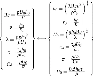
These variables may be arranged into a set of dimen-sionless parameters [11, 12] that govern thin-film rimming flow dynamics namely: Reynolds number, Re; a measure of the filling fraction,ε; gravity parameter,λ; shear parameter, τand capillary number, Ca (or Weber number, We). A defi-nition of these quantities and the two way mapping between the dimensionless space they represent and the dimensional quantities used in this study is illustrated in Figure 3.

A number of numerical challenges have been encoun-tered in previous studies of thin-film rimming flows partic-ularly with regard to shock and pool type solutions involv-ing steep fronts and capillary ripples. A thin-film flow for-mulation for use in a multi-scale CFD model was presented in [10, 13] and is currently implemented in commercial CFD code ANSYS [14]. The Wang model has however so far only been able to reproduce stable smooth solutions and unable to recover stable shock/pool solutions as anticipated from im-posed conditions. In this formulation, the advective terms of the energy and momentum equation are simplified and this is a possible root cause of the numerical difficulties with re-gards to shock/pool solutions in which inertia plays a major role [11, 12].

In mathematical studies such as [8, 9, 15], where a more rigorous formulation is used, including inertia, stable smooth, shock and pool solutions were obtainable. In these

studies, a definitive link between solution stability and sur-face tension was also established. A common practice in these detailed mathematical studies was to retain surface ten-sion terms as a stabilising mechanism and use high surface tension coefficients (corresponding lower Capillary numbers or Higher Weber numers) that are orders of magnitude be-yond what is physically unattainable in engineering condi-tions. For instance, in [11], surface tension was required to be at the first-order of approximation in order to ensure so-lution stability of shock/pool soso-lutions; in reality, this corre-sponds to a surface tension coefficient that is two orders of magnitude higher than is achievable in practice for a typi-cal lubricant described in Table 1. Previously experimental studies by [16] have shown that the presence of even trace amounts of surface-active agents ( about 5×10−3% ) can lead to considerable damping of surface waves and the sup-pression of ripples. This high sensitivity of solutions to sur-face tension further calls into question the validity of simply incorporating high surface tension as a numerical stabilising term as this is likely to affect solution accuracy. There is therefore a need to develop a better understanding of the de-pendency of solution stability on surface tension and its role in the accuracy of the final stable solution in order to iden-tify a remedies for numerical instability in the formulation that do not rely on surface tension based smoothing or lead to unphysical results.

This paper investigates the linkage between surface ten-sion, grid resolution and numerical instability for steady thin-film flow and proposes a solution strategy to ensure numeri-cal stability. In addition, the role plaid by other factors such as inertia formulation, grid resolution and the temporal dis-cretization schemes used in determining solution stability is explored.

Section 2 describes the film formulation used in the present study as well as the proposed inertia corrections and solution approach. The model is then used to carry out a parametric study, reported in section 3, which covers the broad range of film flow regimes and demonstrate the nu-merical difficulties associated with shock/pool solutions as well as the use of artificially high surface tension as a sta-bilising term. A proposed solution strategy is used to over-come these difficulties and obtain stable film solutions within a parameter space that is consistent with the fluid’s physical properties. The verified model and proposed solution strat-egy are finally validated against two test cases; a very Low Re (Re<<1) coating flow experiment by [17], and a mod-erate Re (10<Re<100) experiments for a wavy liquid film falling down an inclined plane by [18].

2 Numerical formulation and solution approach

The thin-film rimming flow in Figure 1 has been ide-alised as a two-dimensional (assuming lateral uniformity) in-compressible Newtonian liquid of density,ρl and viscosity, µl flowing over a solid substrate and with a free-surface

ex-posed to an incompressible Newtonian gas ofρgand

viscos-ity,µg. The film has a spatially varying height, h(s,t)and

flow direction andyis the vertical direction as shown in Fig-ure 1. The film velocityu(s,y,t)may be decomposed into a depth-averaged component ¯u(s,t)and a fluctuating compo-nent ˆu(s,y,t)as

u(s,y,t) =u¯(s,t) +uˆ(s,y,t), (1)

where the mean film speed, ¯u(s,t)is computed as

¯

u(s,t) =1

h

Z h

0

u(s,y,t)dy. (2)

A volumetric film flux may then be computed as, q=

¯

uh. This film flux, q, together with the film height define the film state and are defined by a balance between viscous, gravity (g= (gs,gy)), hydrostatic pressure, surface tension

and film inertia. The resulting film flow dynamics over the solid-substrate are described by the one-dimensional depth averaged continuity and momentum equations given by

∂h

∂t +

∂q

∂s=0, (3)

∂q

∂t +

∂ ∂s

Z h

0

u2dy=−_ρh l

∂Pl

∂s + h

ρl

∂σκ

∂s +gsh+Sτ. (4)

In Equations (3) and (4),Pl= (Pgas−ρgyh), is the film

pressure which has a component from the interfacial gas pressure,Pgasand the film hydrostatic pressure,ρgyh. Pl is

used to compute the film hydrostatic pressure gradient term (S∆P=_ρh

l

∂Pl

∂s) which is the first term on the right hand side

(R.H.S.) of Equation 4.

Surface tension effects are represented in the surface tension term,Sσ=_ρh_l∂σκ_∂s , whereσis the surface tension

co-efficient for the liquid-gas interface, and the interface curva-ture,κ, is estimated according to;

κ=

d2h dx2

1+ dh_dx

!2!1.5. (5)

The third term on the R.H.S. of Equation 4 represents the momentum source term due to film gravitational body forces in the direction of the film flow,Sg=gsh. Finally, the fourth

source term on the R.H.S. of Equation 4,Sτ, represents the

balance of viscous shear forces on the film, including contri-butions from the interfacial shear stress driving the film,τi,

and the wall shear stress resisting fluid flow over the solid

substrate,τw. Using appropriate sub-models to estimateτi

andτw, the viscous source term, Sτ may be computed

ac-cording to:

Sτ=τi−τw

ρl

. (6)

Representative values of the terms of the thin-film equa-tions Equaequa-tions 3 and 4 - the gravity source term (Sg), the

surface tension term (Sσ), the hydrostatic pressure gradient

term (S_∆P), the viscosity term (Sτ) and inertia terms (second

term on the L.H.S. of Equation 4) - have been analysed to determine their relative importance in typical thin-film solu-tions. This is discussed in more detail in section 3 of this paper.

The inertia/convective term of Equation 4 has previously been analytically shown [11, 12] to play an essential role in ensuring solution stability and that without inertia, stable shock/pool solutions are unattainable. The correct represen-tation of the inertia term is therefore key to the development of a robust thin-film formulation. In a number of thin-film models such as [10], a uniform velocity profile is assumed when computing the depth-averaged inertia term, resulting in a “simplified inertia” representation where it is implic-itly assumed that _∂∂_sR₀hu2dy_≈ ∂h_∂u_s¯u¯. In this study, rather than assume a uniform film velocity profile, a more general quadratic film velocity profile is assumed which is consis-tent with the assumption of a laminar uni-directional flow. Higher order cubic and quartic film profiles have also been implemented in order to capture more complex film flows with secondary flow re-circulations. In the falling film cases, the quartic profile was found to give the best agreement with the experimental observations.

2.1 Numerical schemes

Previously the thin-film model [10] has used a semi-implicit solution algorithm where an explicit predictor step is carried out, followed by sequential sub-iterations between the continuity and momentum equations until convergence is attained. In this paper, an explicit MacCormack scheme after [19] has been implemented together with a capillary time-step constraint after [20]. [20] proposed a new capillary time-step constraint derived from a combination of the CFL condition, Nyquist-Shannon sampling theory and the wave Doppler shift due to counter-travelling waves. For a case with a bulk flow of velocityUε, the capillary time step

con-straint may be expressed as [20]:

∆tσ≤ ∆ x √

2Cσ+Uε

, (7)

whereCσis the maximum phase velocity of the resolvable

be given by;

Cσ= s

2πσ ∆x(ρl+ρg)

. (8)

A fully-implicit time-scheme is also implemented, sim-ilar to previous studies such as [11]. In this fully-implicit ap-proach, both the discretised continuity and momentum equa-tions are compiled into a monolithic solution matrix and the resulting non-linear system of equations is solved using MATLAB’s fsolve algorithm or a Newton-Raphson solver.

A fourth-order central difference scheme is used for all spatial derivatives, while a first-order implicit scheme is used for the time discretisation. The solutions are all computed on a uniform base grid of N=600 cells (∆x=1.15mm). A grid-sensitivity study is carried out and results are presented in Section 3.5. In this study, only globally uniform grids have been used.

3 Parametric study

A parametric study has been carried out to investigate the stability behaviour of smooth, shock and pool solutions and its dependence on film surface tension. A characteristic film height in the range of 0.5 - 1.0 mm has been used with uniform interface shear stresses in the range of 1.0 - 10.0 Pa. The interface shear stress and characteristic film height are then varied so as to achieve smooth, shock or pool flow con-ditions within the domain. For the rimming flow simulations, the fluid properties and domain size are described in Tabl1.

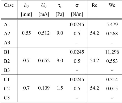
In the parametric study, the surface tension is varied from the physical value of 0.0245 N/m to a value one or-der of magnitude higher. For each of the smooth, shock and pool solution conditions, a simulation is also carried out with the surface tension term ignored. A summary of the simula-tion cases performed is presented in Table 2 along with the corresponding Re and We number.

Cases A1 - A3 were used to test for the sensitivity of smooth flow solutions to the surface tension parameter, while Cases B1 - B5 and C1 - C2 were used to test shock and pool solutions respectively for sensitivity to surface tension. Val-ues of surface tension up to two orders of magnitude larger than the liquid surface tension specified in Table 1 have been tested, which are consistent with the very low capillary num-bers used in [11] for example. The goal of this set of simula-tions, as listed in Table 2 was to explore the range of possi-ble solutions and allow a more detailed understanding of the stability behaviour of these solutions and the role plaid by surface tension and other key terms.

3.1 Smooth solutions

Smooth flow Cases A1, A2 and A3 of Table 2 were suc-cessfully simulated using a full-inertia representation and a full-implicit time scheme. The resulting film thickness and velocity distributions are illustrated in Figure 4a and 4b.

Table 2: Description of simulation cases

Case h0 U0 τi σ Re We

[mm] [m/s] [Pa] [N/m]

A1

0.55 0.512 9.0

0.0245

54.2

5.479

A2 0.5 0.268

A3 -

-B1

0.7 0.652 9.0

0.0245

54.2

11.296

B2 0.5 0.553

B3 -

-C1

0.7 0.109 1.5

0.0245

54.2

0.314

C2 0.5 0.015

C3 -

-These smooth solutions may be characterised as very large wavelength disturbances (of the order of chamber size) in which gravity is the dominant restoring term and surface tension plays a relatively negligible role in the solution. To illustrate this, representative values of some of the key source terms in the thin-film formulation are shown in Figure 4c for a stable smooth solutio. The results in Figure 4c show that in these smooth flow solutions, viscous and gravity forces dominate, while pressure gradient and surface tension play a relatively negligible role.

The surface tension parameter was varied by up to one order of magnitude greater than in the fluid in Table 1 to test for sensitivity. Surface tension was found to have a negligi-ble effect on smooth solution stability or accuracy, with the high surface tension Case A2 showing the exact same result as Case A1. Indeed, a stable smooth film profile was even attainable in Case A3 where no surface tension was present (i.e. when the surface tension term was ignored).

3.2 Shock solutions

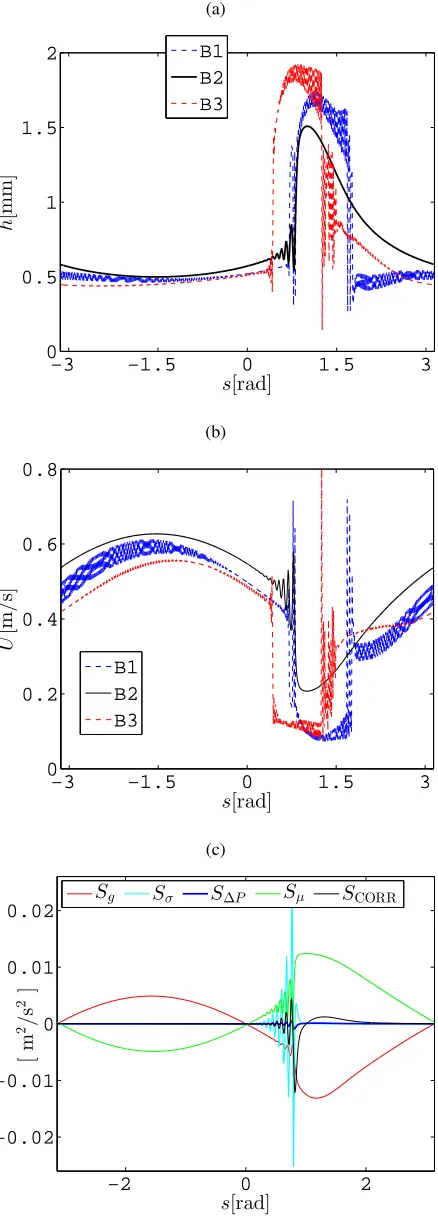
Cases B1, B2 and B3, described in Table 2, represent a region where a shock solution is expected. Surface tension has been varied from the base value of 0.0245 N/m, Table 1, used in Case B1 to Case B3 where surface tension is ig-nored and Case B2 where the surface tension coefficient is one order of magnitude larger than in Case B1. The results in Figures 5a and 5b illustrate that when surface tension is neglected (Case B3) or is of the order of magnitude that is expected for the fluid in Table 1 (Case B1), a stable shock solution is unattainable on the base N=600 grid used. The unstable solutions in these cases are characterised by spuri-ous oscillations which are often accompanied by significant numerical error leading to a loss of mass conservation.

(a)

−2 0 2

0 0.2 0.4 0.6 0.8 1

s[rad]

h

[m

m

]

A1 A2 A3

(b)

−3 −1.5 0 1.5 3

0 0.2 0.4 0.6 0.8

s[rad]

U

[m

/

s]

A1 A2 A3

(c)

−3 −2 −1

−0.01 0 0.01

s[rad]

[

m

2 /

s

2 ]

Sg Sσ S∆P Sµ SCORR

Fig. 4: (a) Film height profiles, (b) velocity distribution and (c) momentum source terms for smooth solutions in Cases A1 - A3.

(a)

−3 −1.5 0 1.5 3

0 0.5 1 1.5 2

s[rad]

h

[m

m

]

B1 B2 B3

(b)

−3 −1.5 0 1.5 3

0 0.2 0.4 0.6 0.8

s[rad]

U

[m

/

s]

B1 B2 B3

(c)

−2 0 2

−0.02 −0.01 0 0.01 0.02

s[rad]

[

m

2 /

s

2 ]

Sg Sσ S∆P Sµ SCORR

in Table 1. The stable shock solution is characterised by a smooth global solution that contains a localised shock region with a sharp change in film profile. Also present upstream of the shock front are small wavelength disturbances which are within the capillary range where surface tension forces are of the same order as gravity forces. For a stable solution, the wavelength of these capillary-gravity waves is sensitive to the surface tension value used. Further discussion on grid sensitivity in Section 3.5 highlights that the presence of these capillary waves and the need to resolve them provides a link between grid resolution, surface tension and solution stabil-ity.

Representative values for the key source terms in the sta-ble shock solutions are shown in Figure 5c. As in the analysis of terms for smooth solutions illustrated in Figure 4c, gravity and viscous terms play a major role in shock solution. How-ever a major difference is the pronounced role played by the surface tension term in the shock solutions where steep gra-dients and very small wavelength disturbances are present. The surface tension term is shown to be of the same order of magnitude as the viscous and gravity terms local to the shock region in contrast to smooth solutions where this term was found to be negligible. The pressure gradient term ex-hibits a slight increase in magnitude in the shock region but remains negligible relative to the other terms.

3.3 Pool solutions

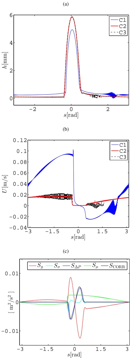
Pool Cases C1, C2 and C3 as described in Table 2, were also simulated using varying surface tension values with the very high surface tension used in Case C2 being an order of magnitude higher than in the typical engineering fluid used in Case C1. Surface tension was neglected in Case C3. Similar to the shock solution results in Figure 5, the pool solution results shown in Figure 6 show that within practical limits on surface tension (or with no surface tension included), stable pool solutions are unattainable on the base grid. However, by increasing surface tension by one order of magnitude on the same grid, stable pool solutions were attainable in Case C2. This stability behaviour demonstrated the stabilising role of surface tension in pool solutions.

Where stable pool solutions exist, they are characterised by a sharp changes in film profile that occurs close to the bottom of the chamber. As the surface shear is insufficient to overcome gravity and distribute the film evenly throughout the domain, the excess oil in the film pools at the bottom of the cylinder. A thinner film is then drawn out of this pool and circulated across the domain.

The representative values of the source terms in the sta-ble pool solution were also analysed and are presented in Figure 6c. In common with the shock case, contributions from gravity, viscous and surface tension terms were found to play a major role in the final stable pool solution. In ad-dition, the pressure gradient term (which was negligible for smooth and shock solutions) is shown to be of the same order as gravity and viscous terms due to the presence of a deep pool to thin-film transition. Therefore in order to simulate realistic pool solutions, the formulation requires gravity,

vis-(a)

−2 0 2

0 2 4 6

s[rad]

h

[m

m

]

C1 C2 C3

(b)

−3 −1.5 0 1.5 3

−0.04 −0.02 0 0.02 0.04 0.06 0.08 0.1 0.12

s[rad]

U

[m

/

s]

C1 C2 C3

(c)

−3 −1.5 0 1.5 3

−0.01 0 0.01

s[rad]

[

m

2/

s

2]

Sg Sσ S∆P Sµ SCORR

cous, surface tension and pressure gradient terms accurately modelled. The findings from this analysis of terms therefore validates previous specifications for an ideal thin-film such as in [10].

3.4 Effect of Weber number

The results presented in sections 3.1 - 3.3 highlight that surface tension plays a significant stabilising role in shock and pool solutions where steep film profiles are present, while it remains negligible for smooth solutions. This sta-bilising role of surface tension for shock pool cases has pre-viously been discussed by, among others, [8], [15] and [11]. In these studies, surface tension was retained as a stabilising term, with high (artificial) surface tension values typically used to ensure stability of the solutions. In the cases so far presented in this paper, stable shock or pool solution on the base grid of N=600 are only attainable using large surface tension values that are at least one order of magnitude higher than those found in a typical engineering application with say oil or water (see Table 1).

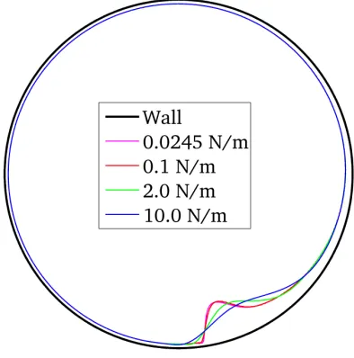
Augmenting the surface tension leads to an artificial smoothing of the solution, creating larger wavelength and low amplitude capillary waves that are easily resolvable on a coarse computational grid. This tends to result in a more sta-ble solution that is easily attainasta-ble. On the other hand, with low surface tension solutions, low wavelength and high am-plitude capillary waves are produced which require a much finer spatial grid resolution. Using a large surface tension coefficients however introduces uncertainty and may lead to excessing damping of the film profile. This is illustrated by the results in Figure 7 where using very high surface ten-sion values (e.g. three orders of magnitude above the physi-cal surface tension) results in a modified shock position and peak film thickness. The use of solution strategies depending on high surface tension should therefore be carried out with caution as significant artificial smoothing of the solution may result.

3.5 Mesh sensitivity

Further more, in addition to confining stable solutions to an unphysical parameter space, these surface tension based stability criteria have been found in the present study to be sensitive to grid resolution. The results of a grid-independence study are illustrated in Figure 8. Results in Figure8a show that for a moderate grid spacing of ∆x=

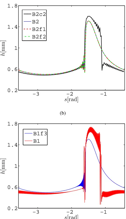
1.15 mm cells, a surface tension coefficient of atleast 0.5 N/m is required to ensure stability of the shock solution in Case B2. Further refinement of the grid to∆x=0.58 mm, Case B2f1, and ∆x=0.29 mm, Cases B2f2, is shown to result in no change to the final stable solution, confirming the independence of the stable solutions to grid refinement. However, using this same surface tension coefficient of 0.5 N/m, if the grid resolution is coarsened to∆x=2.30 mm, as in Case B2c, then the solution is shown to become unstable. Similarly, by using a finer grid of∆x=0.14 mm cells in Case B1f3, which has a relatively low but realistic surface tension coefficient of 0.0245 N/m (consistent with that of oil) it was

Fig. 7: Polar plot of film solution illustrating the artificial smoothing of pool solutions due to the use of very high sur-face tension coefficients.

found that a stable shock solution could be obtained where in Case B1∆x=1.15 mm it could not; this stable shock so-lution was then independent of further grid refinement.

This stability trend suggests that by providing sufficient grid refinement, stable shock/pool solutions may be obtained within practical engineering limits on the surface tension pa-rameter. This minimum grid resolution may be objectively estimated based on the fluid properties and the flow features present in the solution. This is mainly because the grid sen-sitive stability behaviour observed is thought to be rooted in the flow features present in shock solutions, such as steep fronts and capillary waves, which need to be resolved by the computational grid in order to ensure solution stability.

In smooth solutions, only large wavelength disturbances (of the order of the size of the bearing chamber) are present in which gravity is the main restoring force. In these cases, surface tension plays no significant role, except perhaps in stabilising any short wavelength ripples that might emerge during the process of solution. However, as illustrated in Figure 5a, stable thin-film shock/pool solutions are charac-terised by the presence of steep fronts in the solution and short wavelength disturbances that may occur adjacent of the shock front. Figure 9 shows that the wavelength of these disturbances is also sensitive to the value of surface tension used.

(a)

−3 −2 −1

0.2 0.6 1 1.4 1.8

s[rad]

h

[m

m

]

B2c2 B2 B2f1 B2f2

(b)

−3 −2 −1

0.2 0.6 1 1.4 1.8

s[rad]

h

[m

m

]

B1f3 B1

Fig. 8: Results of the grid sensitivity studies for (a) Case B2 (∆x=1.15 mm), Case B2f1 (∆x=0.58 mm), Cases B2f2 (∆x=0.29 mm), Case B2c (∆x=2.30 mm) and (b) Case B1 (∆x=1.15 mm), Case B1f3 (∆x=0.14 mm).

ℓcrit=2π

σ

(ρliquid−ρgas)g !1₂

. (9)

Any given disturbance may be classified according to

if

ℓ << ℓcrit, Capillary wave

ℓ >> ℓcrit, Gravity wave (10)

Using values of surface tension and density shown in Ta-ble 1, the critical wavelength is estimated as,ℓcrit≈10.3 mm.

The main source of instability within shock/pool solution is

0.2 0.4 0.6 0.8 1

0.4 0.8 1.2 1.6

s[rad]

h

[m

m

]

−2 0 2

0 0.5 1 1.5 2

s[rad]

h

[m

m

]

B1f3

B2

Fig. 9: Sensitivity of small-wavelength disturbances in stable Cases B1 (σ=0.0245N/m) and B2 (σ=0.5N/m) to surface tension.

linked to capillary waves whose wavelength is so small that their dynamics are dominated by surface tension which is of the same order of magnitude as gravity (see Figure 5c). In order to obtain a stable shock solution, it is therefore neces-sary that sufficient grid resolution be provided to resolve the expected short wavelength disturbances, otherwise the solu-tion becomes numerical unstable. Results from simulasolu-tions performed in the present research suggest an empirically de-rived maximum grid size,∆xmaxmay be estimated as

∆xmax≈

ℓc

60. (11)

This mesh sensitivity partly explains the success of past approaches such as [11] (also demonstrated in Sections 3.2 and 3.3) where a high surface tension value is used to ensure numerical stability of the solution on a grid of moderate spac-ing spacspac-ing. A direct consequence of numerically increasspac-ing the surface tension coefficient is that the critical wavelength,

ℓcdefined by Equation 9, is also increased. Consequently, a

coarser grid resolution may be successfully used to resolve the key feature and obtain a stable solution. However, for a fixed surface tension coefficient corresponding to the fluid used in this study, Equations 9 and 11 suggest that the grid should be of N=400 (∆x_≈0.17mm) or finer in order to en-sure numerical stability of shock solutions. The same would be valid for a deep pool simply because, starting from a uni-form film profile, the solution may transit through a shock condition before reaching a steady pool state. If sufficient resolution is not provided to resolve the solution transition through a shock, a stable pool solution is then unlikely to be reached.

3.5.1 Proposed mesh-based solution strategy

stable shock/pool solutions within a constrained parameter space, it is suggested that;

firstly, sufficient grid refinement to resolve capillary waves is provided;

secondly, in order to rapidly obtain the steady solution, a solution may be obtained using artificially high surface tension values which may then be progressively relaxed to match fluid properties (Table 1) in the final solution.

The grid resolution requirement is determined accord-ing to Equations 9 and 11. Although a uniform grid has been used for all simulations in this paper, the grid size cri-teria may be applied to the shock region only using a non-uniform/adaptive meshing approach. For the low surface tension cases, in order to improve convergence times, an ini-tial solution is obtained quickly using a high surface tension value to start with; the surface tension is then progressively relaxed until the conditions in Table 1 are reached. This strat-egy is shown to be grid independent provided the minimum grid resolution suggested by Equation 11 is provided. Fur-ther grid refinement beyond this level was shown to have no impact on the solution as shown in Figure 8a.

The proposed grid-refinement solution strategy is there-fore identified as a more objective alternative to the surface tension smoothing strategy. Surface tension based smooth-ing strategies, when chosen as the preferred approach due to grid size considerations, should be used with caution and it is recommended that a grid and surface tension sensitiv-ity study always be performed as film solutions can be very sensitive to surface tension [16], [22].

3.6 Effects of inertia representations

As has been discussed in Section??for thin-film com-putations, the simplification of the non-linear inertial term can lead to significant inaccuracies or numerical instability of the solution. However this effect has hitherto not been in-vestigated, and by presenting the thin-film formulation in a form that is easily convertible into a full-inertia formulation (as in [11]) or the simplified inertia formulation (as in [10]), the effects of inertia representation on smooth, shock and pool solutions can be assessed.

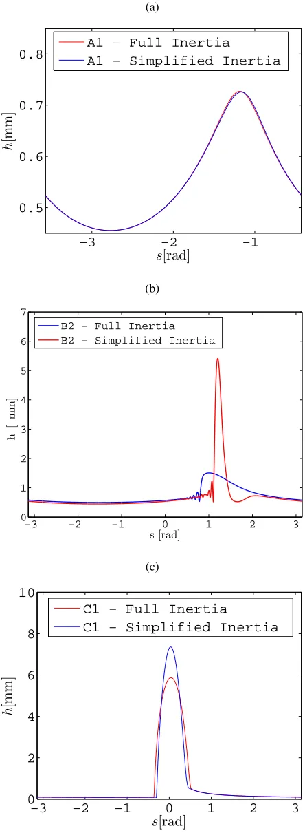
Case A1 (smooth solution), Case B2 (shock solution) and Case C2 (pool solution) were simulated using both a simplified- and a full-inertia representation in order to as-sess the role this plays in solution stability. The results of this sensitivity test for inertia representation are illustrated in Figure 10.

Stable smooth solutions for Case A1 were obtained for both the simplified-inertia and full-inertia as shown in Figure 10a. A comparable performance confirms that inertia terms and correspontingly their representations do not play a major role in smooth solutions. The inertia correction source term is negligible in these smooth solutions as shown for represen-tative values of the smooth solution source terms in Figure 4c.

The inertia representation sensitivity results for a shock solution, Case B1, are shown in Figure 10b. Results for the

(a)

−3 −2 −1

0.5 0.6 0.7 0.8

s[rad]

h

[m

m

]

A1 − Full Inertia

A1 − Simplified Inertia

(b)

−3 −2 −1 0 1 2 3

0 1 2 3 4 5 6 7

s [rad]

h[mm]

B2 − Full Inertia B2 − Simplified Inertia

(c)

−3 −2 −1 0 1 2 3

0 2 4 6 8 10

s[rad]

h

[m

m

]

C1 − Full Inertia

C1 − Simplified Inertia

simplified inertia case show significantly larger shock height than those obtained when the corrective source term is in-cluded to recover a full inertia formulation. Inertia effects affect the accuracy of shock solution considerably with the simplified inertia formulation shown to introduce significant errors. However, it should be noted that a stable solution is still obtainable using simplified inertia, hence inertia repre-sentation appears to affect solution accuracy but not the over-all stability. The representative values for the source terms in the shock case with full inertia show that the corrective source term is of the same order of magnitude as surface ten-sion, gravity and viscous terms.

Similar findings to the shock solutions are observed for pool solutions in Case C2 as shown in Figure 10c. The cor-rective source term in the case of these pool solutions is shown in Figure 6c to be of comparable order as viscous, gravity, surface tension and pressure gradient terms.

Computational results demonstrate that provided the proposed solution strategy is employed together with an im-plicit time scheme, a simplified inertia approach primar-ily effects accuracy but not stability of smooth, shock or pool solutions. In addition, the successful recovery of full-inertia using a corrective source term is demonstrated as a non-intrusive method of including full-inertia in existing simplified-inertia formulations such as [11].

3.7 Effects of time-scheme

Results so far presented have been carried out using a fully-implicit time scheme as described in section 2.1. The results demonstrate that using a fully-implicit time scheme, stable smooth, shock and pool solutions are obtained, even in cases where simplified inertia representations are used. For the rimming flow cases where the steady solution is a station-ary wave front, the capillstation-ary time constraint proposed by [20] was found not to be a necessary condition for numerical sta-bility.

With the explicit schemes, very low Courant-Friedrichs-Lewy (CFL) numbers (less than 1E-2 ) were required in order to get stable solutions for the rimming flow problem, regard-less of the inertia formulation used. The solution exhibits significant mass loss as well as spurious oscillations.

While the implicit solver was found to give a consider-able saving in computational cost for solutions involving sta-tionary wave fronts (e.g. the case of a rimming flow shock solution) this was not the case for travelling wave fronts (e.g. falling film cases) where the capillary time-step con-straint [20] was a necessary condition for stability. As a re-sult of the low CFL requirement, the explicit MacCormack scheme was found to give a more computationally efficient solution to travelling wave cases than the implicit scheme. The choice of an efficient time-scheme is therefore depen-dent on the physics of the flow being simulated.

4 Model Validation

The proposed model and solution strategy has been vali-dated against available experimental datasets from literature.

Two test cases are selected; firstly a thin-film coating flow inside a rotating cylinder by [17] and secondly a wavy liquid film flowing down an inclined plane by [18].

4.1 Coating flow simulations

In the coating flow experiment reported in [17], a small amount of viscous liquid completely coats a horizontal rotat-ing cylinder. The cylinder was rotated at a very slow speed and high viscosity liquid used so as to ensure that the flow remained within the creeping flow regime (Re<<1). The resulting film solution is therefore the result of a balance be-tween viscous, inertia, gravity and surface tension forces.

The experiment [17] was performed in a 0.27 m long Plexiglass cylinder of 0.05 m diameter. These dimensions have also been used in the thin-film simulations presented here. The liquid used was a combination of TritonX-100, ZnCl2and water with a viscosity of 4.0 Pa.s, density of 1172

kg/m3 and surface tension of 0.031 N/m. In all the exper-iments, the Reynolds number, Re= (Ωh02)/ν) was always

less than 10−2, whereh0is the mean thickness of the film.

For different combinations of filling fraction,F, and ro-tational parameterα= (Ων/gR)1/2_{, the film thickness}

mea-surements are taken along the circumference of the cylinder in the central portion of the cylinder using a needle attached to the end of a rod. The experimentally measured film thick-ness were then integrated over the cylinder circumference to obtain the local filling fraction,F, at a given axial location as in [17].

Table 3 gives a summary of the three experimental cases simulated using the thin-film model. The results from these simulations are plotted together with corresponding exper-imental measurements in Figure 11. Results show good agreement between the thin-film model and the experimental measurements by [17] for the creeping flow (Re<<1) con-ditions of the experiment. The thin-film model is therefore proven to give a reliable prediction for film thickness in low Re rimming flow conditions.

Table 3: Selected coating flow experimental cases [17] sim-ulated using the thin-film model

Case Rotational Pa-rameter,α

Filling frac-tion,F

Re

Case 1 0.0341 0.1625 1.03E-3

Case 2 0.0376 0.1198 6.08E-4

Case 3 0.0568 0.1126 1.16E-3

4.2 Wavy falling liquid film flow

(a)

(b)

(c)

Fig. 11: Experimental and thin-film predicted film thickness distributions for (a)

up of aqueous solutions of glycerine (54 % by weight) with density 1136.2 kg/m3, dynamic viscosity 0.00713 Pa.s and surface tension of 0.067 N/m. The flow inlet is acoustically excited in order to generate small amplitude monochromatic oscillations. For moderate frequencies, as the film flows down the plane, these oscillations evolve into large ampli-tude solitary waves with steep fronts which are preceded by capillary ripples. These solitary waves are physiologically similar to the shock type rimming solutions discussed in Sec-tion 3.2 and offer a validaSec-tion case for the performance of the thin-film model in these types of solutions. For the case simulated, an inlet forcing frequency of 1.5 Hz and Re = 29 were evaluated using both simplified and full inertia approx-imations.

Figure 12 shows the simulation results. The simplified inertia formulation is shown to significantly over-predict the peak film thickness although the wave separation is accu-rately predicted. Using the full inertia formulation, both the peak film thickness and wave separation are shown to give good agreement to the experimental data from [18].

Fig. 12: ETFM predictions for solitary waves travelling down a 6.4◦slope with Re = 29 and inlet forcing frequency of 1.5Hz. ETFM model results for both simplified and full in-ertia representations are shown together with equivalent ex-perimental measurements from [18]

5 Conclusion

A depth-averaged Eulerian Thin Film modelling ap-proach has been successfully applied to the numerical simu-lation of smooth, shock and pool type solutions. In this for-mulation, gravity, viscous, pressure gradient, surface tension forces and inertia are accounted for.

In smooth solutions, both pressure gradient and surface tension terms are shown to be negligible compared to gravity and viscous terms. While in shock and pool solutions, sur-face tension and pressure gradients are found to play a signif-icant role in the solutions and are of the same order as gravity and viscous terms. Smooth solutions have been shown to be insensitive to the surface tension parameter while the numer-ical stability of shock/pool solutions has been shown to be dependent on the value of surface tension used and the pro-vision of sufficient grid refinement to resolve steep fronts and capillary waves present. The wave-length of the disturbances in this capillary wave region are shown to be dependent on the surface tension coefficient used, with high surface ten-sion leading to large wavelength and low amplitude capillary waves and vice-versa.

Solutions strategies that rely on using large surface ten-sion values (low Ca or high We) to guarantee stability do so by damping the waves in the capillary region to one that is resolvable on the available grid. This however introduced additional uncertainty as surface tension smoothing may pro-duce un-physical results due to excessive damping. As an alternative, this study has demonstrated grid-based solution strategy for obtaining numerically stable solutions within the constraints imposed by the fluid properties has been success-fully.

The effect of inertia representation has also been ex-plored and stable shock, smooth and pool solutions are shown to be obtainable using both the simplified and full in-ertia formulations. However for shock and pool solutions, the simplified inertia formulation affects solution accuracy in the shock/pool region - leading to an over-predicted peak film thickness.

An assessment of implicit, and explicit time schemes has revealed that for stationary wave fronts such as in the case of rimming flows, fully implicit schemes offer considerable computational saving and the capillary time-step constraint is not a necessary condition for stability in these cases. How-ever, for travelling wave fronts as in the case of falling wavy films, the capillary time-step constraint must be observed and this results in very low CFL for which the explicit MacCor-mack scheme is more efficient than a full implicit scheme.

Acknowledgements

The research leading to these results has received fund-ing from the European Union?s Seventh Framework Pro-gramme under grant agreement No 314366 (E-BREAK project).

This document is property of the E-BREAK Consor-tium, it must not be diffused without the prior written ap-proval of the authors.

References References

[1] OBrien, S. B. G., and Schwartz, L. W., 2002. “The-ory and modeling of thin film flows.”.Encyclopedia of surface and colloid science, pp. 5283–5297.

[2] WITTIG, S., GLAHN, A., and HIMMELSBACH, J., 1994. “Influence of high rotational speeds on heat-transfer and oil film thickness in aeroengine bearing

chambers”. JOURNAL OF ENGINEERING FOR GAS

TURBINES AND POWER-TRANSACTIONS OF THE ASME,116(2), APR, pp. 395–401. 38th International Gas Turbine and Aeroengine Congress and Exposition, CINCINNATI, OH, MAY 24-27, 1993.

[3] Glahn, A., and Wittig, S., 1996. “Two phase air/oil flow in aero engine bearing chambers: Characteriza-tion of oil film flows”.JOURNAL OF ENGINEERING FOR GAS TURBINES AND POWER-TRANSACTIONS OF THE ASME,118(3), JUL, pp. 578–583. 40th In-ternational Gas Turbine and Aeroengine Congress and Exhibition, HOUSTON, TX, JUN 05-08, 1995. [4] Chandra, B., Simmons, K., Pickering, S.,

Colli-cott, S. H., and Wiedemann, N., 2013. “Study of gas/liquid behavior within an aeroengine bearing

chamber”. JOURNAL OF ENGINEERING FOR GAS

TURBINES AND POWER-TRANSACTIONS OF THE ASME,135(5), MAY.

[5] Hirt, C., and Nichols, B., 1981. “Volume of fluid (vof) method for the dynamics of free boundaries”. Journal of Computational Physics,39(1), pp. 201 – 225. [6] Gao, D., Morley, N., and Dhir, V., 2003.

“Numeri-cal simulation of wavy falling film flow using{VOF}

method”. Journal of Computational Physics, 192(2), pp. 624 – 642.

[7] Miyara, A., 2000. “Numerical simulation of wavy liq-uid film flowing down on a vertical wall and an in-clined wall”. International Journal of Thermal Sci-ences,39(911), pp. 1015 – 1027.

[8] Ashmore, J., Hosoi, A. E., and Stone, H. A., 2003. “The effect of surface tension on rimming flows in a partially filled rotating cylinder”. Journal of Fluid Mechanics, 479, pp. 65–98.

[9] Benilov, E. S., Lapin, V. N., and OBrien, S. B. G., 2012. “On rimming flows with shocks”.Journal of Engineer-ing Mathematics,75, pp. 49–62.

[10] Wang, C., Morvan, H. P., Hibberd, S., Cliff, K. A., Anderson, A., and Jacobs, A., 2012. “Specifying and benchmarking a thin film model for oil systems appli-cations in ansys fluent”. In In ASME Turbo Expo 2012: Turbine Technical Conference and Exposition, pp. 229-234. American Society of Mechanical Engineers. [11] Kay, E. D., Hibberd, S., and Power, H., 2014. “A

depth-averaged model for non-isothermal thin-film rimming flow”. International Journal of Heat and Mass Trans-fer,70, p. 10031015.

[12] Williams, J., 2008. “Thin film rimming flows subject to droplet impact at the surface”. PhD thesis, The Uni-versity of Nottingham.

2011. “Thin film modelling for aero-engine bearing chambers”. In ASME 2011 Turbo Expo: Turbine Tech-nical Conference and Exposition, pp. 277-286. Ameri-can Society of Mechanical Engineers, 2011.

[14] ANSYS INC, 2015.ANSYS Fluent 16.0 User’s Guide. [15] Villegas-Diaz, M., Power, H., and Riley, D. S., 2005. “Analytical and numerical studies of the stability of thin-film rimming flows subject to surface shear”. Jour-nal of Fluid Mechanics,541, pp. 317 – 344.

[16] Taliby, S., and Portalski, S., 1961. “The optimum con-centration of surface active agent for the suppression of ripples”.Trans. lnstn Chem. Engrs,39, pp. 328 – 336. [17] Tirumkudulu, M., and Acrivos, A., 2001. “Coating

flows within a rotating horizontal cylinder: Lubrica-tion analysis, numerical computaLubrica-tions, and experimen-tal measurements”. Physics of Fluids (1994-present), 13(1), pp. 14–19.

[18] Liu, J., and Gollub, J. P., 1994. “Solitary wave dynam-ics of film flows”. Physics of Fluids (1994-present), 6(5), pp. 1702–1712.

[19] MacCormack, R., 2003. “The effect of viscosity in hy-pervelocity impact cratering”. Journal of Spacecraft and Rockets,40, Sept., pp. 757–763.

[20] Denner, F., and van Wachem, B. G., 2015. “Numeri-cal time-step restrictions as a result of capillary waves”. Journal of Computational Physics,285, pp. 24 – 40. [21] Lamb, H., 1994. Hydrodynamics (6th ed.). Cambridge

University Press. ISBN 978-0-521-45868-9.