Stability and cycles in a cobweb model with heterogeneous expectations

STABILITY AND CYCLES IN

A COBWEB MODEL WITH

HETEROGENEOUS EXPECTATIONS

L

L

S

S

C

T

University of Queensland

We investigate the dynamics of a cobweb model with heterogeneous beliefs, generalizing the example of Brock and Hommes (1997). We examine situations where the agents form expectations by using either rational expectations, or a type of adaptive expectations with limited memory defined from the last two prices. We specify conditions that generate cycles. These conditions depend on a set of factors that includes the intensity of switching between beliefs and the adaption parameter. We show that both Flip bifurcation and Neimark–Sacker bifurcation can occur as primary bifurcation when the steady state is unstable.

Keywords:Bounded rationality, Cobweb model, Flip bifurcation, Neimark–Sacker bifurcation

1. INTRODUCTION

In relation to economic modeling, there has been a lengthy and continuing debate about formation of expectations. Although the rational expectations hypothe-sis plays a major role in dynamic macroeconomic research, papers that model expectations relaxing that assumption are increasing, but few of these inves-tigate the dynamics in any detail. The cobweb model of Brock and Hommes (1997) first gave a satisfying exposition on both accounts, that is, a rigorous

This is a revised version of Lasselle et al. (2003). Comments by two anonymous referees and an associate editor helped to improve an earlier version of the paper and are gratefully acknowledged. We thank the seminar participants at the University of St. Andrews, the University of Manchester, the University of Swansea, Heriot-Watt University, the European University Institute, the University of Edinburgh, and the participants of the 2002 Money, Macro, and Finance Conference, of the 2003 Royal Economic Society Conference, of the 2003 WEHIA Conference for comments. We are particularly indebted to Valentyn Panchenko and Cars Hommes, affiliated to the CeNDEF in Amsterdam. They gratefully embedded our model in the software E&F Chaos allowing us to derive the diagrams. All errors are ours. This work was done while Laurence Lasselle was Jean Monnet Fellow at the Economics Department of the European University Institute, Florence, Italy. Address correspondence to: Laurence Lasselle, School of Economics and Finance, St. Andrews, Fife, KY16 9AL, United Kingdom; e-mail: [email protected].

c

foundation for heterogeneous beliefs and a systematic dynamical study. The expectation formation arises from rational choice between various costly fore-casts. The concept of adaptively rational equilibrium dynamics (ARED), in which market equilibrium dynamics is coupled to the choice of prediction of learn-ing strategies, is introduced. Brock and Hommes then showed that this type of expectation formation can generate inherent instability for the ARED, lead-ing to possible complex motions. The present paper further develops this ap-proach by considering a different set of forecasts and aims at characterizing such instability.

Over the past decade, a growing number of papers have dealt with the role of het-erogeneous expectations in generating instability (Chiarella and He, 1998, 2001; Franke and Neseman, 1999; Goeree and Hommes, 2000; Hommes, 1991). While economic implications of these studies are obvious for some specific markets,1 most papers, including ours, are based on the simple cobweb model, as it is one of the most tractable models involving market dynamics.

The framework and the economic import of these papers, including ours, are close to those of Brock and Hommes (1997).2

Let us first consider the framework. Expectation formation is modeled as a rational economic decision. Indeed, producers choose between two methods of predicting prices depending on their performance, namely a costly sophisticated predictor and a costless unsophisticated predictor.3_{The predictor’s performance is} defined as the net realized profits in the most recent period less the cost associated with using the predictor. Depending on this performance, each producer may at every period switch from one predictor to another. For producers as a whole, this switching process, which is perfectly endogenous, may occur at various levels of intensity.

Let us now turn to the economic meaning of this class of models (Branch, 2002; Brock and Hommes, 1997; Lasselle et al., 2003). Under the previous assumptions on the expectation formation and the ARED concept, the instability of the steady state is generated by a simple but powerful mechanism which can be intuitively described as follows.

On the one hand, when the price is close to its steady-state value, very few agents use the most sophisticated predictor, since its cost exceeds the benefits of its forecast. Therefore, the distance between the current price and its steady-state value grows large over time.

On the other hand, while its cost is significant, the sophisticated predictor provides a better net return when the current price is far from its steady-state value. Thus, the distance between the two prices gets smaller over time.

Let us illustrate this mechanism4 _{in the model of Brock and Hommes (1997).} Suppose that at timetthe current price is close to but greater than its steady-state value and the vast majority of agents use the na¨ıve expectations predictor. As a result, the supply att+1 is mainly evaluated frompt, but the demand is computed

same reasoning is true for the following period. The current price att+2 will be greater than its steady-state value.

Consequently, price oscillations are endogenously generated in the steady-state neighborhood.

The immediate steps in research can then be either to look for stability conditions for convergence of the price dynamics and their consequences in the model, as did Branch (2002), or to characterize the steady-state instability, as pioneered by Brock and Hommes (1997). It is indeed well known that any complete dynamical analysis should begin with that characterization, as it can lead to complicated dynamical phenomena studied from bifurcation. When a bifurcation occurs, the qualitative properties of the dynamical system in the vicinity of steady state have been modified following a small change in value of one of the parameters of the model. At the critical value of the parameter, there exists one steady state. However, if the parameter increases beyond that critical value, even if the perturbation is small, then there exist cycles.

Brock and Hommes (1997) showed that this mechanism could lead to highly complex dynamics. They focused on a bifurcation route to chaos. On this route, the primary bifurcation can only be a Flip bifurcation; that is, the equilibrium time paths exhibit attracting cycles of period 2.

The main contribution of our paper is to show that this mechanism can lead not only to the possibility of stable cycles of period two, but also to attracting limit cycles through primary bifurcations. Indeed, we show that when the steady state is unstable, supercritical Flip bifurcation as well as supercritical Neimark– Sacker bifurcation can occur for a set of parameters. The existence of these two types of attracting cycles is directly linked to our definition of the expectation functions.

While Brock and Hommes (1997) assume that costly rational expectations are competing with costless na¨ıve expectations, we replace the latter by cost-less adaptive expectations. More precisely, we assume that adaptive expecta-tions are a weighted average of the last two prices. This relaexpecta-tionship, which is crucial for our results, is a reasonable alternative possibility to the re-lationships assumed by Brock and Hommes (1997) and by Branch (2002), for instance. It was already present in Hommes’s cobweb model (1998) with homogenous and adaptive expectations.5 _{Allowing for adaptive expectations,} we consider its implications using the evolutionary framework of Brock and Hommes (1997).6

We can then imagine that beyond two periods they do not keep the information about prices. Second, agents could also believe that the prices observed more than two periods ago would have no impact (or so little impact) on future prices that it is not necessary to take account of that information. Third, one could conjecture that the extra cost in keeping and taking that information into account would exceed the extra benefit to be obtained. Therefore, it would be “econom-ically rational” not to take these earlier prices into account in the prediction function.

Given the existing literature derived from Brock and Hommes (1997), our model allows us to derive two new results.

First, the model of Brock and Hommes (1997) becomes a special case of our model. Indeed, the na¨ıve expectations they consider correspond to our adaptive expectations when all weight is put on the most recent price. As we consider an expectation function with two lags, the dimension of the dynamical system of our model increases from 2 to 3. Due to this change, we are able to demonstrate the existence of a new type of primary bifurcation, namely a primary Neimark–Sacker bifurcation.9

Second, our conclusion is more cautious than that of Branch (2002). Branch (2002) considers a more generalized setting than Brock and Hommes (1997) and us. Indeed, he examines in detail the stability properties of the cobweb model when agents can choose between three predictors: the rational expectations predictor, the na¨ıve predictor, and adaptive beliefs. On pp. 77–78, he studies a model close to ours where agents choose between a costly predictor and a costless adaptive predictor defined as a weighted average of the most recent price and the most recent forecast. This scheme requires as much memory as our scheme based on a weighted average of the two most recent prices. One of his main conclusions (Theorem 8, p. 77) states that the stability conditions of the steady state are broader when adaptive expectations put “enough” weight on the past. As our model is simpler than his, our conclusion is more specific. First, the stability zone is wider when the agents base their adaptive expectations on both past prices with more weight on the most recent price. In other words, the “size” of the stability region is nonmonotonic in the adaption parameter. Second, the instability of the steady state may lead to stable cycles. On the one hand, these cycles may appear when the agents put “enough” weight on the current price (cycles occurring through a Flip bifurcation). On the other hand, stable cycles can also occur when the agents put “reduced” weight on the most recent price (cycles occurring through the Neimark–Sacker bifurcation). We conclude that the adaptive predictor is stabilizing relative to na¨ıve expectations and there exists a critical parameter value related to the switching process that can induce a bifurcation regardless of the weight on past information in the adaptive predictor.

2. THE COBWEB MODEL WITH RATIONAL VERSUS ADAPTIVE EXPECTATIONS

We present an extension of the model of Brock and Hommes (1997) that focuses on the case of rational versus na¨ıve expectations. The only two changes to their framework are the following. On the one hand, we consider the introduction of an adaptive expectation function with two lags rather than na¨ıve expectations. On the other hand, the analysis is based on the relative number of agents using ratio-nal expectations compared to the number of agents using adaptive expectations, denoted byn1. Although the second change is just a matter of presentation, the first change, through small, leads to significant differences in results. To make the results comparable with these of Brock and Hommes (1997), we follow their setup closely.

Supply decisions are made by choosing the output that maximizes expected profits subject to the one-period production lag. That is,

max

q

p_te₊₁q−c(q),

wherec(q)is the cost function, which is increasing inq.

Price expectations, pe_t+1, are formed by choosing a predictor from a set of expectation functions. Given this heterogeneity in expectation formation, market supply is a weighted sum of the supply decisions of the heterogeneous agents. The weights are simply the proportion of agents using a specific predictor. That is, in our model each agent chooses between two predictors,Hj∈ {H1, H2}, where each predictor depends upon a vector of past pricesPt=(pt, pt−1, . . . ,p0). The fractions of agents using one of the two predictors,nj,t(pt,H(Pt−1))depend on

the current price and on the vectors of previous predictors:

H(Pt₋1)=(H1(Pt₋1), H2(Pt₋1)). Therefore, market equilibrium is given by the equation

D(pt₊1)= 2

j=1

nj,t(pt,H(Pt₋1)) S(Hj(Pt)),

whereD(.)is the demand function andS(.)is the supply function.

To keep the model analytically tractable, we assume linear demand and supply. Therefore letD(pt)=F −Bpt be the demand andS(Hj(Pt))=bHj(Pt)be the

supply, withF, B, b∈R₊.

Without loss of generalization of the stability properties, we setFequal to zero. Market equilibrium is determined by the condition

where the two predictor functions are defined as

H1(Pt)=pt+1 with costC≥0, (2)

H₂(Pt)=τpt+(1−τ )pt−1 with 0< τ <1 and no cost. (3)

Each period, after observing the new price and assessing the accuracy of their fore-casts, producers update their prediction of the next period’s price. The evolution of the proportion of agents using a particular predictor is given by

nj,t+1=Exp(βUj,t+1)

₂

j=1

Exp(βUj,t+1). (4)

Uj,t+1is a measure of the welfare associated with a certain predictor.

The variableβ parameterizes preferences over profits. The largerβ, the more likely a producer is to switch to an expectation with slightly higher returns. Brock and Hommes call this the “intensity of choice” parameter. Assume that the measure of the welfare is equal to realized net profits in the last period; then we obtain

Uj, t+1=πj[pt+1,H(Pt)],

where

πj[pt+1,H(Pt)]=pt+1S[Hj(Pt)]−c{S[Hj(Pt)]} −Cj.

Cj is the fixed cost associated with Hj. The cost of production is a simple

quadratic cost functionc(q)=q2/(2b). The profit functions for producers using each predictor are respectively

π1(pt₊1, pt₊1)= b 2p

2

t+1−C, (5)

π2(pt+1, pt, pt−1)=

b

2[τpt+(1−τ )pt−1][2pt+1−(τpt+(1−τ )pt−1)]. (6)

Plugging these into (4) leads to the law of motion for the two predictors,

n1, t+1=Exp

β

b 2p

2

t+1−C Zt+1, (7)

n₂,t+1=Exp

βb

2[τpt+(1−τ )pt−1] [2pt+1−(τpt+(1−τ )pt−1)] Zt+1,

(8)

whereZt₊1= 2

The cobweb model with rational and adaptive expectations is a system (S) of nonlinear difference equations that governs the law of motion of price,

pt₊1=φ (pt, pt₋1, n1, t), (9)

and the law of motion of the proportion of agents using the rational expectation predictor,

n1, t+1=ϕ(pt, pt−1, n1, t), (10)

where

φ (pt, pt−1, n1,t)=A(n1,t)[τpt+(1−τ ) pt−1],

A(n₁,t)=b(n1,t −1)/(B+b n1,t),

and

ϕ(pt, pt₋1, n1,t)

= 1

1+Exp−β₂{b[(τpt+(1−τ )pt−1)2(A(n1,t)−1)2]−2C}

.

Since (9) and (10) are, respectively, a second-order difference equation and a first-order difference equation, the system (S) can be rewritten as a system of three first-order difference equations (S):

ht+1=pt, (11)

pt+1=φ (ht, pt, n1,t), (12)

n₁,t+1=ϕ(ht, pt, n1,t). (13)

The stability or the instability of the steady state issued from the system (S) formed by equations (11), (12), and (13) can be directly investigated by looking at the Jacobian matrix of (S) taken at the steady state. These stability properties will be studied in the following section.

3. STABILITY AND CYCLES

A simple computation shows that the system (S) has a unique steady stateE = (0,0,n¯1(β)=1/[1+Exp(β C)]). To ease the presentation, let us assume that C=0 or C=1. When C=0, the agents have free access to the sophisticated predictor.

PROPOSITION 1. Assume that the slopes of the supply and the demand satisfy b/B >1. When the information costs are nil, the steady state is E = (0,0,n¯1(β)=1/2)and is always locally asymptotically stable.

The proof is left to the reader.

PROPOSITION 2 (Local Stability of the Steady State). Letb/B>1andC=1. There exists a uniqueE=(0,0,n¯1(β)),wheren¯1(β)=1/(1+Expβ)with the

following properties:

(i) ∃β1such that:

(a) ∀0≤β < β1and∀2/3< τ <1,E is locally asymptotically stable.

(b) ∀β > β1and for all2/3< τ <1,E is locally unstable.

(ii) ∃β2such that:

(a) ∀0≤β < β2and∀τ∈(0,1/2∪1/2,2/3),E is locally asymptotically stable.

(b) ∀β > β2and∀τ∈(0,1/2)∪(1/2,2/3),E is locally unstable.

Proof. See Appendix.

PROPOSITION 3 (Primary Bifurcations of the Steady State). Letb/B >1and

C=1.

(i) Fix2/3< τ <1. Whenβ=β1,the system undergoes a supercritical Flip

bifur-cation.

(ii) Fix τ∈(0,1/2)∪(1/2,2/3). When β=β2, the system undergoes a Neimark–

Sacker bifurcation. Moreover,the Neimark–Sacker bifurcation is supercritical on someτ∈(0,1/2)∪(1/2,2/3).

(iii) Whenτ=1/2,the system is in strong resonance1:3. (iv) Whenτ=2/3,the system undergoes a codim-2bifurcation.

Proof. See Appendix.

The dynamical analysis depends on a set of parameters composed of the adaption parameter,τ, the intensity of choice, β, and the slopes of the demand and the supply,Bandb. For specific combinations of these parameters, the steady state can lose its stability, giving birth to periodic equilibria; that is to say, the system undergoes a primary bifurcation and stabilizing fluctuations in prices can appear. We are able to prove analytically when these bifucations arise.

FIGURE1.Local stability of the steady state.

predictor to the other predictor is balanced with the adaptation parameter. On the other hand, for specific values of the intensity of choice, regardless of the weight on past information in the adaptive predictor, stable cycles in prices can appear.

Consequently, the substitution of na¨ıve expectations by adaptive expectations in the cobweb model with heterogeneous expectations can not only create a more stable environment but also foster the possibility of stabilizing cycles.

The following figures illustrate our propositions and facilitate the understanding of our findings.

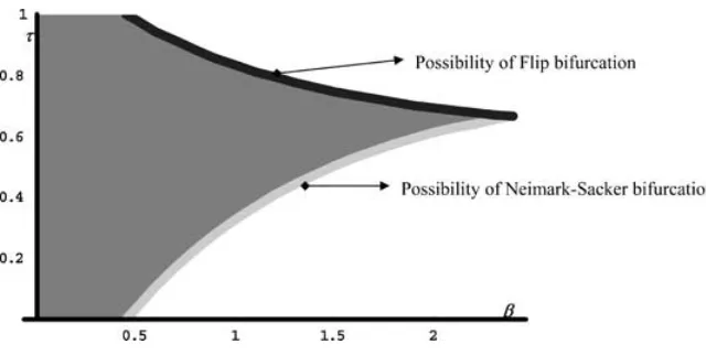
Figures 1 and 2 show how the stability of the steady state depends on the parameters values. Up to three curves are drawn: the eigen curve, the flip curve, and the NS curve. On each curve,βis at its critical value, to which is associated a specific value ofτ. The eigen curve consists of parameter values for which the eigenvalues of the Jacobian matrix evaluated at the unique steady state change from real to complex. The flip curve consists of parameter values for which one of the eigenvalues is equal to –1. It represents the possibility of Flip bifurcation as a primary bifurcation. The NS curve consists of parameter values for which complex eigenvalues have moduli equal to 1. It represents the possibility of Neimark–Sacker bifurcation as a primary bifurcation. The flip curve and the NS curve intersect when τ = 2/3. Finally, the unique steady state is locally asymptotically stable in the shaded region, where all the moduli of the eigenvalues are less than 1.

FIGURE2.Local stability of the steady state whenB=0.3 andb=1.35.

real or complex. On the other hand, it is the coefficient in the law of motion of the prices.

We can point out two facts. First, whatever the value of the adaption parameter, the steady state can be asymptotically stable, but the size of the stability of the region is nonmonotonic inτ. Second, the system can undergo a bifurcation, but the possibility of primary bifurcation rests on specific values betweenτ andβ. Indeed the two parameters are jointly dependent; that is, to the critical value of the intensity of choice corresponds a specific value of the adaptive parameter. Let us develop these facts from Figure 2.

Figure 2 illustrates the nonmonotonic relationship betweenβandτ. It plots the flip and NS curves in the(β, τ )-plane for specific values of the parameters of the demand and the supply,B=0.3 andb=1.35. It shows overall that the adaptive expectations (whenτ∈(0,1))are less destabilizing for the market than the na¨ıve expectations (τ=1).

Whatever the value of the adaptation parameter, the unique steady state can be locally asymptotically stable for small values of the intensity of choice. But as the intensity of choice is increasing, there is a need for a more balanced weighting between the two prices to ensure this stability. Note that this “more” balanced weighting is not a completely balanced weighting. Indeed, the most recent information must count for around 2/3 in the adaptive expectations func-tion. So our evolutionary framework adds a new feature. There exists a favorable trade-off between information and the speed of movement between the predic-tors. More balanced information captured on each side of the steady state can increase the speed of movement between predictors without destabilizing the market.

steady state. Second, our cheap predictor rests on two periods, so it captures the most recent information on each side of this unique steady state. Third, adaptive expectations dampen the oscillations.

Now suppose that at timetthe current price is close to but greater than its steady-state value and a vast majority of agents use the adaptive expectations predictor. The supply in t+1 is mainly evaluated from pt and pt−1, but the demand is

computed from the current price int+1. As the dynamics in the cobweb model is inherently oscillatory, the current price int+1 will be less than the steady-state value. But it will be higher than if na¨ıve expectations were the costless predictor. The same reasoning is true for the following period. The current price int+2 will be greater than its steady-state value, but less than the value that can be found if na¨ıve expectations were the costless predictor. Consequently, price oscillations are more dampened in our model in the steady-state neighborhood. The second parameter of our model, the intensity of choice, which inherently fosters divergent dynamics in the model, can thus increase without damaging the stability. We may say that the process of switching predictors in this model enhances stability of the model.

As we shall see in the following figures, as the set of parameters varies, the local stability of the steady state can be transformed and for fixed sets of parameters it can lead to stabilizing cycles.

Figure 3 assembles several graphs and illustrates Proposition 3(ii). Notably, we can see a limit cycle for specific values of the parameters in the(p(t−1), p(t ))-plane (recall thatp(t−1)=h(t )). The initial conditions areh0 =0.2,p0 =1, andn1,0 = 0.5; the parameters are as follows:τ=0.628,β−2.11272,C =1, B =0.3,b=1.35.

One could then wonder what happens to the dynamics of the current priceptor

of the current proportion of agents using the rational expectations predictorn1,t

when the intensity of choiceβincreases (for a givenτ).

Let us first consider a value ofτ greater than 2/3. Figures 4a and 4b show the bifurcation diagrams ofp (4a) and n1 (4b) with respect toβ for a fixed value of τ (τ=0.8). As β increases between 1.5 and 10, the system can undergo a variety of period-doubling. The primary bifurcation occurs aroundβ =1.18. The unique steady state in prices loses its stability and becomes a cycle of period 2; the uniqueness ofn₁can disappear. Asβtakes higher values, there is a possibility of periodic attractors.

Let us now consider a lower value of τ (τ=0.6)and assess the dynamical behavior of our variables asβ takes larger and larger values.10

Figures 4c and 4d show the bifurcation diagrams ofp (4c) andn1 (4d) with respect toβ. Asβincreases between 1.5 and 10, the system can undergo a variety of bifurcation. The primary bifurcation occurs aroundβ=1.94. The unique steady state in prices loses its stability and becomes a limit cycle. The uniqueness ofn1 disappears.

FIGURE3.Limit cycle in prices and ¯n1=0.107867, τ=0.628, β=2.11272, C=1, B=

0.3, b=1.35.

from the sophisticated predictor to the cheap predictor becomes more and more irregular as the intensity of choice increases.

The phenomena first shown by Brock and Hommes (1997) exists in our model and confirms the possibility ofa rational route to randomness.

FIGURE3.Continued.

expectations predictor, causing a speedy convergence towards the steady state. Note that the change between the two patterns is irregular and each pattern is more or less lengthy.

Second, the experiments show that the Lyapunov characteristic exponent is positive for large values of the intensity of choice when the adaptation parameter takes some high or low values, implying the possibility of chaotic behavior in our model.

4. CONCLUDING COMMENTS

A

ND

CYCLES

IN

A

C

OBWEB

M

ODEL

643

FIGURE5.τ=0.6, C=1, B=0.3, b=1.35,β−7.

may, by themselves and when their formation is modeled as an economic de-cision, be sufficient to generate endogenous fluctuations in this evolutionary framework.

FIGURE5.Continued.

NOTES

1. See for instance Frankel and Froot (1990) for concerns related to the foreign exchange market. 2. See also Brock and Hommes (1995).

3. A basic but necessary assumption used in the literature on this topic is the local instability of the steady state when all agents use the cheap predictor.

4. Brock used the Samuelson’s boat parable to illustrate this mechanism (refer to Brock’s interview by Woodford (2000)).

5. There is no endogenous switching process; the supply curve is nonlinear.

6. A similar formulation is also used in the cobweb model of Chiarella and He (1998).

7. The reference to bounded rationality is quite common in the literature on heterogeneous expec-tations. See for instance Tisdell (1996) or Hommes (2000).

8. The type of rational economic decision-making underlying our model is more akin to that of Baumol and Quandt than to that of Simon. The former treats the problem as an optimizing one. The latter considers it as a “satisficing” one. However, our model includes elements of both ideas.

9. See Proposition 3. For a mathematical exposition of bifurcations, we refer to Kuznetsov (2000).

REFERENCES

Azariadis, C. (1993)Intertemporal Macroeconomics. Cambridge: Blackwell.

Baumol, W.J. and R.E. Quandt (1964) Rules of thumb and optimally imperfect decisions.American Economic Review54, 23–46.

Branch, W.A. (2002) Local convergence properties of a cobweb model with rationally heterogeneous expectations.Journal of Economic Dynamics and Control27, 63–85.

Brock, W.A. and C.H. Hommes (1995) A Rational Route to Randomness. TI 95-87, Timbergen Institute.

Brock, W.A. and C.H. Hommes (1997) A rational route to randomness.Econometrica65(5), 1059– 1095.

Chiarella, C. and X.-Z. He (1998) Learning about the cobweb.Complex Systems98, 244–257. Chiarella, C. and X.-Z. He (2001) Asset Price and Wealth Dynamics under Heterogeneous

Expec-tations. Paper presented at the second CeNDEF Workshop on Economic Dynamics, University of Amsterdam, January 4–6, 2001.

Franke, R. and T. Neseman (1999) Two destabilizing strategies may be jointly stabilizing.Journal of Economics69(1), 1–18.

Frankel, J.A. and K.A. Froot (1990) Chartists, fundamentalists, and trading in the foreign exchange market.American Economic Review80(2), 181–185.

Frouzakis, C.E., R.A. Adomaitis, and I. Kevrekidis (1991) Resonance phenomena in an adaptively-controlled system.International Journal of Bifurcation and Chaos1, 83–106.

Goeree, J.K. and C.H. Hommes (2000) Heterogeneous beliefs and the non-linear cobweb model.

Journal of Economic Dynamics and Control24, 761–798.

Hommes, C.H. (1991) Adaptive learning and road to chaos.Economics Letters36, 127–132. Hommes, C.H. (1998) On the consistency of backward-looking expectations: The case of the cobweb.

Journal of Economic Behaviour and Organization33, 333–362.

Hommes, C.H. (2000) Cobweb dynamics under bounded rationality. In E.J. Dockner et al. (eds.),

Optimization, Dynamics, and Economic Analysis—Essays in Honor of Gustav Feichtinger, pp. 134–150. Berlin: Physica-Verlag.

Kuznetsov, Y.A. (2000)Elements of Applied Bifurcation Theory, 2nd ed. Applied Mathematical Sci-ences 112, New York: Springer-Verlag.

Lasselle, L., S. Svizzero, and C. Tisdell (2003) Heterogeneous Expectations, Dynamics, and Stability of Markets. Working paper 0308, University of St. Andrews.

Simon, H.A. (1957)Models of Man. New York: Wiley.

Tisdell, C. (1996)Bounded Rationality and Economic Evolution. Cheltenham, UK: Edward Elgar. Woodford, M. (2000) An interview with William Brock.Macroeconomic Dynamics4, 108–138.

APPENDIX

Proof of Proposition 2. We just need to study the stability properties of the steady stateE=(0,0,n¯1(β)=1/(1+Expβ)). The steady state is asymptotically stable when

all the absolute values of the real eigenvalues or all the moduli of the complex eigenvalues of the Jacobian matrix atEare less than 1 (Azariadis, 1993).

The Jacobian matrix atEis

J= 

A(n¯1(β))(0 1−τ ) A(n¯1(β))(τ )1 00

0 0 0

In what follows, we will denote ¯n1(β)by ¯n1, keeping in mind that the relative weight of

agents using rational expectations depends on the intensity of choiceβ.

(i) IfA(n¯1)τ2+4(1−τ ) <0⇔A(n¯1) <−4(1−τ )/τ2, then there are three

eigenval-ues, 0 and

λ1,2=

A(n¯1)τ∓

A(n¯1)[A(n¯1)τ2+4(1−τ )]

2 .

Study ofλ1:

λ1<−1⇔

A(n¯1)τ−

A(n¯1)[A(n¯1)τ2+4(1−τ )]

2 <−1

⇔A(n¯1)τ+2<

A(n¯1)[A(n¯1)τ2+4(1−τ )].

IfA(n¯1)τ+2<0⇔A(n¯1) <−2/τ, this inequality is always true and thenλ1<−1

whateverτ.

Let us now assume thatA(n¯1)≥ −2/τ and let us find the conditions for which

−1< λ1<0. We have

−A(n¯1)τ−2<−

A(n¯1)[A(n¯1)τ2+4(1−τ )]

⇔A(n¯1) >−1/(2τ−1) ifτ >1/2

(note that−1/(2τ−1) >−2/τwhenτ >2/3)

⇔(−3τ+2)/[τ (2τ−1)]<0 ifτ >2/3.

So we have shown that when−2/τ <−1/(2τ−1) < A(n¯1) <−4(1−τ )/τ2and τ >2/3, then−1< λ1<0.

Study ofλ2: It is easy to check that−1< λ2<0.

(ii) IfA(n¯1)τ2+4(1−τ ) >0, then there are three eigenvalues: 0 and

λ1,2=

A(n¯1)τ±i

−A(n¯1)[A(n¯1)τ2+4(1−τ )]

2 .

Study of the modulus:

|λ1,2| =

A(n¯1)τ

2 2

+ 1

4{−A(n¯1)[A(n¯1)τ

2+₄₍₁−_{τ )]}}

=−(1−τ )A(n¯1)|λ1,2|<1⇔A(n¯1) >−1/(1−τ )

(note that−1/(1−τ ) >−4(1−τ )/τ2_{when 0< τ <2/3).}

Proof of Proposition 3(We Follow Kuznetsov (2000)). Our system (S) is three-dimensional and needs to be rewritten so that the steady state is at the origin:

ht+1 =pt,

pt+1 =φ (ht, pt, n1,t),

Let us denotemt =n1,t−n¯1. Then the system (S) becomes the following system (S1):

ht+1=pt, (A.1)

pt+1=φ(ht, pt, mt+n¯1), (A.2)

mt+1=ϕ(ht, pt, mt+n¯1)−n¯f=ψ(ht, pt, mt) . (A.3)

The steady state is then(0,0,0).

Let us denote (S1) as a discrete–time dynamical system:

x→f (x) (A.4)

We can write this system as

˜

x=J x+F (x), x∈R3_{, (A.5)}

whereJis the Jacobian matrix of (A.4) at the steady state andF (x)=O(x2_{)is a smooth}

function. Let us represent its Taylor expansion in the form

F (x)= 1

2B(x, x)+ 1

6C(x, x, x)+O(x

4_),

whereB(x, y)andC(x, y, z)are multilinear functions.

Let us first consider the Flip case (Proposition 3i). In that case,A(n¯1)= −1/(2τ−1)

andτ∈(2/3,1).

The Jacobian matrixJof (A.4) at the steady state is

J =   

0 1 0

(τ−1)/(2τ−1) −τ/(2τ−1) 0

0 0 0

  .

There are three eigenvalues: 0,−1, and (τ −1)/(2τ −1). The corresponding critical eigenspace is one-dimensional and spanned by an eigenvectorq∈R3_{such thatJ q= −q,}

whereqT _=(1/√_2,−1/√_{2,0). Lets∈R}3_{be the adjoint eigenvector; that is,J}T_{s= −s,} whereJT_{is the transposed matrix ofJ. Normalizeswith respect toqsuch thats, q =1,} wheresT ₌√_{2/(2−3τ )(1−τ,2τ−1,0).}

The bilinear functionB (x, y), defined for two vectorsx=(x1, x2, x3)Tandy=(y1, y2, y3)T∈R3, can be partitioned into three elements,

B (x, y)=    

0

x3B1p,3y1+x3Bp2,3y2+x1Bp1,3y3+x2Bp2,3y3

x1B1m,1y1+x2Bm1,2y1+x1Bm1,2y2+x2Bm2,2y2    ,

where B1,3

p =(1−τ )A(n¯1),Bp2,3=τ A(n¯1), Bm1,1=(τ−1)

2 σ, B1,2

m =τ (1−τ ) σ, and B2,2

m =(τ )

2_{σ, withσ=βbExp[β](A(n¯}

1−1))2/(1+Exp[β])2and

A(n¯1)=

2τ b (2τ−1)

1 B+bn¯1

.

Following Kuznetsov, the map (A.5) can be transformed to the normal form,

˜

ε= −ε+χ (0)ε3 _+O(ε4_),

where

χ (0)= 1

6s, C(q, q, q) − 1

2s, B(q, (J−Id)

−1

B(q, q)) = −1 4

(1−2τ )4 (2−3τ )σ A

_(n¯

f).

We denote by Id the Identity matrix.

Thus, the critical normal form coefficientχ (0), which determines the nondegeneracy of the Flip bifurcation and allows us to predict the direction of bifurcation of the two-period cycle, is always positive whenτ >2/3. Therefore, the Flip bifurcation is nondegenerate and always supercritical.

Let us now consider the Neimark–Sacker case (Proposition 3(ii)). In that case,A(n¯1)=

−1/(1−τ )and 0< τ <1/2 and 1/2< τ <2/3. The Jacobian matrixJof (A.4) at the steady state is

J = 

−01 −τ/(11−τ ) 00

0 0 0

 .

There are three eigenvalues: 0 and

λ1,2= − τ 2(1−τ )±i

√

(2−τ )(2−3τ )

2(1−τ ) =Re(λ)±iIm(λ).

Jhas a simple pair of eigenvalues on the unit circleλ1,2 =e±iθ0withπ/2< θ0< πand θ0=2π/3. Letq∈C3be a complex eigenvector corresponding toλ1,

J q=eiθ0_{q, Jq¯}=_e−iθ0_q,¯

qT _{=(1,Re(λ)+iIm(λ),0) and ¯q}T _{=(1,Re(λ)−iIm(λ),0).Introduce also the adjoint} eigenvectors∈C3_{having the properties}

JT_s=e−iθ0_{s and J}T_s¯=eiθ0_s¯

and satisfying the normalization

s, q =1,

wheres, q =3_i=1s¯iqiis the standard product inC3,

¯

sT = 1

2 Im(λ)i(−Re(λ)+iIm(λ),1,0).

Following Kuznetsov, we know that in the absence of strong resonances, that is,

eikθ0=_{1, fork}=_1,2,3,4,

the map (A.5) can be transformed into

˜

withα(0)=Reκ(0), which determines the direction of the bifurcation of a closed invariant curve. This real number can be computed by the following invariant formula:

α(0)= 1 2Re{e

−iθ0_{[s, C(q, q,q)¯} +_{2s, B(q, (Id}−_{J )}−1_B(q,q))¯

+ s, B(q, (e¯ 2iθ0_Id−_{J )}−1_{B(q, q))]}}_.

Therefore,

α(0)=1 2Re

A(n¯1)σ

(Re(λ)τ )((Im(λ)τ )2−3L2)+L(L2−3(Im(λ)τ )2)

+(L2+(Im(λ)τ )2)2 2

,

whereL=τ−1−τ2_{/[2(τ−1)].}

The coefficientα(0)is always negative whenτ∈(0, 0.203817)∪(0.59299,2/3. There-fore, the Neimark–Sacker bifurcation is nondegenerate and supercritical on these intervals. When τ = 0.5, Lasselle et al. (2003) establish thatA(n¯f) = −2 andθ0 = 2π/3.

The stationary equilibrium then undergoes a strong resonance 1:3 (see Kuznetsov (2000), p. 397).