Antonio Ramires Fernandes
A Thesis Submitted for the Degree of PhD
at the
University of St Andrews
1997
Full metadata for this item is available in
St Andrews Research Repository
at:
http://research-repository.st-andrews.ac.uk/
Please use this identifier to cite or link to this item:
http://hdl.handle.net/10023/13468
Robustness and Generalisation:
Tangent Hyperplanes and Classification
T rees
A thesis submitted to the
UNIVERSITY OF ST. ANDREWS
for the degree of DOCTOR OF PHILOSOPHY
By
Antonio Ram ires Fernandes
All rights reserved
INFORMATION TO ALL USERS
The quality of this reproduction is dependent upon the quality of the copy submitted.
In the unlikely event that the author did not send a com plete manuscript and there are missing pages, these will be noted. Also, if material had to be removed,
a note will indicate the deletion.
uest
ProQuest 10167232
Published by ProQuest LLO (2017). Copyright of the Dissertation is held by the Author.
All rights reserved.
This work is protected against unauthorized copying under Title 17, United States C ode Microform Edition © ProQuest LLO.
ProQuest LLO.
789 East Eisenhower Parkway P.Q. Box 1346
-the record of work carried out by me and that it has not been submitted in any previous application for a higher degree.
Date: Signature of candidate: ^
K /%
I was admitted as a research student under Ordinance No. 12 in 1991 and re registered as a candidate for the degree of Doctor of Philosophy in 1992; the higher degree study for which this is a record was carried out in the University of St. Andrews between 1991 and 1996.
Date: Signature of can ^d ate:
In submitting this thesis to the University of St. Andrews I understand that I am giving perm ission for it to be made available for use in accordance with the regulations of the University Library for the time being in force, subject to any copyright vested in the work not being affected thereby. I also understand that the title and abstract will be published, and that a copy of the work may be made and supplied to any bona fide library or research worker.
I hereby certify that the candidate has fulfilled the conditions of the R esolution and R egulations appropriate for the D egree o f D octor of Philosophy in the U niversity o f St. A ndrews and that the candidate is qualified to submit the thesis in application for that degree
The issue o f robust training is tackled for fixed m ultilayer feedforw ard architectures. Several researchers have proved the theoretical capabilities of M ultilayer Feedforw ard netw orks but in practice the robust convergence of standard m ethods like standard backpropagation, conjugate gradient descent and Quasi-Newton methods may be poor for various problem s. It is suggested that the common assum ptions about the overall surface shape break down when m any individual com ponent surfaces are com bined and robustness suffers accordingly.
A new m ethod to train M ultilayer Feedforw ard netw orks is presented in which no particular shape is assumed for the surface and where an attempt is made to optim ally combine the individual components of a solution for the overall solution. The method is based on computing Tangent Hyperplanes to the non-linear solution manifolds. At the core of the method is a mechanism to minimise the sum of squared errors and as such its use is not limited to Neural Networks. The set of tests performed for Neural Networks show that the m ethod is very robust regarding convergence of training and has a powerful ability to find good directions in weight space.
A ck n ow led gem en ts
This thesis would not have been possible without the help of Mike W eir, my supervisor. I w ould like to thank M argarida Fernandes, my m other, for lending me her Macintosh for what turned out to be a long period of time, and M argaret and Helen, from the Computer Science Division.
Last, but definitely not least, I would like to thank Carmen Roriz, my wife, and Tiago Sam uel, my son, for putting up with me and for encouraging me u n c o n d itio n a lly .
1.1. Brains and Computers...1
1.2. The Neurocomputing vs. The Symbolic Approach ...2
1.3. General Structure of Feedforward Neural Nets ...6
1.4. Issues in Neural Nets ... 7
1.4.1. The Architecture ... 8
1.4.2. Generalisation...9
1.4.3. Robustness...
..11
1.5. Thesis Structure...12
1.6. Notation... 13
1.6.1. Equations... 13
1.6.2. Figures and Tables...14
2. An Introduction to Artificial Neural Nets ... 15
2.1. The ADALINE and the Delta Rule... 19
2.1.1. A graphical perspective of the ADALINE ...24
2.1.2. Conclusion... 27
2.2. Multilayer Feedforward Networks ...28
2.2.1. Architecture Definition ...28
2.2.2. Feeding a Pattern to the Net ... 30
2.2.3. A Graphical Perspective for M ultilayer
Feedforward Nets ...
32
2.3. Standard Backpropagation ...44
2.3.1. The Backpropagation Rule ...44
2.3.2. A Graphical Perspective of Backpropagation ...49
2.3.3. Momentum...52
2.3.4. Conclusion...
53
2.4. Conjugate Gradient Descent...
54
2.5. Other Minimisation Techniques ...57
3. Tangent Hyperplanes ...61
3.1. An Alternative View of Goal Weight States ...61
3.1.1. The Solution Manifold View for Single Layer Nets ...63
3.1.1.1. Minimising Euclidean Distance to a Set of Solution
Manifolds... 64
3.1.1.2. A Least Squares Approach to Minimise Euclidean
Distance ... ... .65
3.1.1.3. Conclusion...69
3.1.2. Non-linear Systems of Equations ...70
3.1.3. Conclusion...71
3.2. Linear Approximation to Non-linear Solution Manifolds ...71
3.2.1. Conclusion...77
3.3. Tangent Hyperplanes as Linear Approximations ...77
3.3.1. Nets with a Single Output Unit ... .78
3.3.2. Nets with Multiple Output Units... 83
3.4. Tangent Hyperplanes with line Search ... 86
3.5. Tangent Hyperplanes with Subgoals ...
88
3.5.1. Candidate Subgoal Evaluation... 90
3.5.2. Candidate Subgoal Setting Using Output Measures...95
3.5.3. Candidate Subgoal Setting Using Weight Space
Measures... ... ... 98
3.5.4. The Approach Taken...
103
3.5.5. Subgoal Computation... 104
3.5.6. The Algorithm...
107
3.6. Conclusion...109
4. Normalisation Issues ...Ill
4.1. The Effects of Normalisation in linear Systems ...
I l l
4.2. The Single Layer Net Case ... 113
4.3. The Multilayer Net Case...115
4.4. Normalisation Including an Error Term ...118
5.1. The XOR problem...127
5.1.1. Standard Backpropagation with Subgoals ...128
5.1.2. Standard Backpropagation...
132
5.1.3. Tangent Hyperplanes with line Search ...134
5.1.4. Tangent Hyperplanes with Subgoals ...136
5.1.5. Conclusion...140
5.2. The 5 Bit Parity Problem ...141
5.2.1. Standard Backpropagation... 142
5.2.2. Tangent Hyperplanes ... 143
5.3. The 2 Spirals Problem...149
5.4. A Function Approximation Problem ...
154
5.4.1. Standard Backpropagation... 155
5.4.2. Tangent Hyperplanes ... 155
5.4.3. Conclusion...157
5.5. Conclusion ...157
6. Classification T rees... 160
6.1. linearly Separable Problems ... 161
6.1.1. 2-D Input Space...164
6.1.1.1. Reducing the Dimensionality of the Problem ...164
6.1.1.2. Reducing the Search Space by Half ...173
6.1.1.3. Summary and Geometrical Interpretation ...
177
6.1.2. n-D linear separable problems ...178
6.2. linearly inseparable problems ... 182
6.3. Classification Trees...187
6.4. Solving the 2 Spirals Problem with Classification Trees ...193
6.5. Conclusion...195
7. A Mechanism for Generalisation ...197
7.2. Relation to Other W ork...207
7.3. An Implementation using Classification Trees ...208
7.4. Experiments... 211
7.4.1. The 2 Spirals Problem...211
7.4.2. Randomly Generated Training Sets ...214
7.4.2.1. The Quarter Circle Problem... 215
7.4.2.2. The line Problem ...217
7.5. Conclusions... 219
8. Conclusion...221
8.1. Future Work...
224
8.1.1. Robust Training...224
8.1.2. The Classifier...225
8.1.3. Generalisation Framework ... 225
Appendix A. Thesis Software Manual ...226
A.I. Fixed Multilayer Feeforward Architectures ...226
A. 1.1. Simnet : Interactive Simulator ... 226
A. 1.1.1. The Context Menu...
229
A.I. 1.2. Starting Training ...
231
A. 1.1.3. The Remaining Options Available in the Main
Menu ...
233
A. 1.1.4. I/O Maps : How to visualise them... 234
A.1.2. Batch Testing ...235
A.I.2.1. Testing TH with Subgoals...235
A.I.2.2. Testing TH with Subgoals Extensively ... 238
A.I.2.3. Testing TH with line Search ... 241
A. 1.2.4. Testing Backpropagation ... 243
A.2. Classification Trees and Generalisation Framework ...245
A.2.1. Building the Classification Tree ... 246
A.2.2. Testing the Classification Tree ... ...247
C hapter 1. Introduction
1. Introduction
1.1. Brains and Com puters
Although nowadays computers o f the digital symbolic type are said to be very powerful machines the human brain still outperform s them very easily in a variety of tasks. In fact, brain and symbolic computers seem to complement each other, or as Caudill and Butler (1989) put it, "brains and computers are handy things to have". They are good at fundam entally different things.
Caudill and B utler (1989) present two examples that show a fundam ental difference between a symbolic computer and a person. The first is dividing a seven digit number by another number. This task is extrem ely difficult for the average hum an person, it requires follow ing a com plicated sym bolic algorithm and there is plenty room for errors to occur. On the other hand an electronic calculator can do it very rapidly and w ithout any errors. The second exam ple involves recognising a human face in a crowded room. In this case, the task is fairly simple for a human but extremely hard even for the m ost advanced symbolic computer running the most advanced software.
It is the awareness of this discrepancy in abilities that today leads scientists to research on how the brain operates and ultimately how to emulate the brain's non-sym bolic behaviour in a computer.
The brain is a fascinating 'm achine'. Its capabilities are astonishing by any standards. Hertz, Krogh and Palmer (1991) list some of the features that the brain possesses:
• It is flexible. It can easily adjust to a new environm ent by 'learning' - It doesn't have to be programmed in Pascal, FORTRAN or C;
• It can deal w ith inform ation that is fuzzy, p robabilistic, noisy or in c o n s is te n t;
• It is highly parallel.
T h ese fe a tu re s are h ig h ly d e sira b le in c o m p u ta tio n a l sy stem s. Neurocomputing is the science that attempts to incorporate these features in a computational system. In §1.3 a more detailed analysis is done comparing the classical com putational system s based on the sym bolic paradigm with n e u ro c o m p u tin g .
A lthough in the early ages o f neurocom puting researchers inside the com m unity w ere careful to m ake their neurocom puting m odels plausible from a biological point of view, nowadays neurocom puting is no longer strongly attached to biological factors. A rough and simple modelling may be sufficient to extract at least some of the previously m entioned properties. If initially neurocom puting was used m ainly as a com putational model for the brain, today neurocom puting is used for many practical applications like forecasting, pattern classification, etc., and therefore this detachm ent from biology is justifiable.
H ow ever since the initial inspiration for neurocom puting was the brain, some biological terms rem ain in use. For instance, a neurocom puting system is a network of units usually referred to as neurons, and some researchers still talk about synapses when referring to the connections between neurons.
1.2. The Neurocom puting vs. The Sym bolic Approach
C hapter 1. Introduction
exam ple o f the classical approach expert system s are presented. E xpert system s are based on a know ledge base, an inference engine and a user interface. The knowledge base is a problem specific set of IF-THEN rules that describes the particular problem being dealt with. The inference engine is the module that consults the knowledge base and acts upon the information in it. The user interface links the inference engine to the external e n v ir o n m e n t.
To create a knowledge base for an expert system the knowledge needed to solve the problem m ust be incorporated into the knowledge base. However such knowledge is in some situations incomplete. The factors that influence the problem m ight not be fully known. Furtherm ore, according to G allant (1993), in many cases the knowledge is very hard to translate into rules. For instance, in the general case hum ans are very good at recognising faces. However writing a set of IF-THEN rules to distinguish two persons based on their photographs is by no means a trivial task.
G allant (1993) says that the process of construction and debugging a knowledge base is the main problem in building expert systems. Gallant goes even further saying that once the knowledge is extracted from the expert(s), the knowledge base is almost certain to be incomplete or inconsistent.
In some cases an expert is still needed; however the expert's role is different from the classical sym bolic approach. For instance in forecasting problem s, the expert does not need to specify symbolic rules that model the process as in the traditional approach. Instead, the role of the expert is m ainly to identify the variables and targets which may be important to the forecast and provide a significant set of examples of how the system should behave. It is up to the neurocomputing system to learn how to relate the variables in order to obtain a correct forecast.
A neurocomputing system learns by example; a large enough set of examples must be created to teach the system. The neurocomputing system extracts the rules in the asymbolic sense outlined by Denker et. al, (1987) needed to solve the problem during the learning process based on the examples presented.
The structure of the examples, called patterns from now on, depends on the neurocom puting paradigm being used. Some paradigms require the pattern to have two components, an input vector, or input pattern, and an output vector or target. These patterns can be seen as the desired behaviour for the neurocom puting system to learn, i.e. they specify w hat the system should respond, the target, when prom pted with a query, the input pattern. Other paradigms require only the input pattern. In these cases it is up to the system to learn how to separate the different examples into classes.
C hapter 1. Introduction
pattern and a respective specific target output pattern. In this way, each time the neural net is presented with an input pattern an error can be computed based on the difference between the output given by the net and the specific target. The error is then fed to the system so that the system can evaluate its perform ance and correct its behaviour accordingly.
A nother im portant feature of neurocom puting is the capability o f dealing w ith incom plete or even partially incorrect inputs. This further enhances the perform ance o f neurocom puting system s when com pared with classical com puting approaches. Furtherm ore, in the general case, a neurocom puting approach is capable of providing a sensible answer in geom etric terms to inputs it has never seen before. For exam ple, in the face recognition problem , when a neurocom puting system receiv es a slig h tly blurred photograph it may still recognise the face in it.
The above m entioned features give an edge to neurocom puting system s over sym bolic system s such as expert system s for some problem s. There are however areas in which expert systems, for example, are clearly better suited than neurocom puting. Expert system s are able to tell the user how they reached a certain output from an input state in m eaningful term s. The symbolic rules used to achieve the output can be listed, reassuring the user, or at least justifying why the expert system achieved a certain output. This is not always possible with the neurocom puting approach. The knowledge base in a neurocomputing approach is not as easy to consult as the set of IF-THEN rules that forms the knowledge base of expert systems. The knowledge base in a neurocomputing approach is defined in more detail in §1.3.
example enables a conclusion to be drawn as to which inputs from the input example had more influence on the output obtained.
In order to combine the best features of both systems a hybrid approach is possible. For an example, Gallant (1993) shows how a knowledge base of a neurocom puting system can serve as a knowledge base for an expert system that perform s classification tasks.
1.3. G eneral Structure of Feedforward Neural Nets
A neurocomputing system in its most simple form is a single neural network. From now on, unless stated otherwise, this thesis deals only with one class of neural netw orks: feedforw ard netw orks.
A multilayer feedforward net can be defined as a box with a set of inputs and a set of outputs. Inside this box are a number of simple processing units called
neurons that com m unicate with each other through weighted links. Signals are sent to a neuron either from the inputs or from other neurons through the weighted links, hereafter called weights. These signals are combined in some way to become the excitation of the neuron. The excitation may be then further processed to obtain an activation which in turn may be further processed to obtain an output for the neuron. The output of a neuron is then sent to other neurons or to the outputs of the box. Since the network must be feedforward there must be no cyclic paths in the network.
The set of weights specifies not only which neurons connect to which but the strength of the respective connection. The outputs obtained when the box is presented with an input pattern are a function of these weights. Therefore the set of weights can be seen as the internal state of the box.
C hapter 1. Introduction
input/output relation. In such situations the box has to change its internal state to perform the correct input/output mapping. A learning rule is used for this effect, gradually changing the internal state of the box so that the initial input/output relation perform ed by the neural net becom es the desired input/output association.
To illustrate how learning occurs the supervised learning mode is presented since this is the learning mode used in this thesis.
The learning process is often an iterative process. A set of patterns, each pattern made of an input vector and a target, is presented to the box. An error can then be computed for the set of patterns comparing the outputs obtained for each pattern with the targets for the respective pattern. Afterwards the learning rule adjusts the internal state of the box so that the error is decreased. The set of patterns is presented again and again, and the internal state is modified each time, until a sufficiently low error is obtained.
The internal state of a neural net can be seen as representative o f the knowledge a neural net contains. Therefore it makes sense to talk about the knowledge base of a neural net when referring to its internal state. Hence the knowledge base of a neural net is the set of connections present in the neural net as well as their strengths. The knowledge is represented in a num erical fashion as opposed to the sym bolic approach used in expert system s. This is the main reason why it is so hard to extracts reasons for action from the knowledge base of a neural net.
1,4. Issues in Neural Nets
The issues discussed here are the ones relevant to this type of net. R esearchers in N eural N etw orks face three m ain issues: the internal structure o f the neural net, called the architecture, the generalisation ability, and the robustness o f the learning regim es. In the follow ing subsections each of these issues is discussed.
1.4.1. The Architecture
The first issue that faces som eone trying to use neural nets to solve a particular task is how to define the architecture of the net, i.e. what is the number of neurons needed and how to connect them to perform a certain task .
One possible approach to avoid having to determ ine the precise num ber of neurons needed is based on algorithms that consider the architecture to be a variable. This approach is capable of finding an appropriate architecture as part o f the learning process, therefore elim inating to a certain extent the problem of knowing a priori the num ber of neurons needed to solve a problem . These algorithm s, in the general case, w on't find the m inim al necessary architecture to solve a problem but rather an architecture that is sufficient to solve the problem of realising the training set. Hertz, Krogh and Palm er (1991) divide these algorithm s into three broad categories : Pruning, weight decay, and growing algorithm s.
C hapter 1. Introduction
ex trem es b ecau se th e larg er the num ber o f n eu ro n s th e m ore com putationally expensive the training process will be.
Regarding the topology, W eight Decay, proposed by Lang and Hinton (1990), rem oves unused connections from the network. The principle is to diminish the weight values after each iteration so that weights that are not reinforced will tend to zero. W eights below a threshold value are removed. As mentioned before for the pruning algorithm s, w ith this technique having a priori knowledge about what is a large enough architecture to solve the problem , without falling into extremes, is also requested for good performance.
Growing algorithm s start with few neurons and add neurons to the network as needed to realise the desired I/O relation. For examples of these techniques see Mezard and Nadal (1989), Fahlman and Lebiere (1990), and Frean (1990). A possible disadvantage of these methods is that they may end up with a much larger architecture than needed to solve the problem.
It is also possible to combine these methods, for instance one can use a grow ing algorithm to construct an initial architecture that solves the problem and afterwards use a pruning algorithm or w eight decay to remove the unnecessary hidden units.
1.4.2. Generalisation
The ability to generalise is very important in a neural network. If one wanted a lookup table for a particular training set then using a neural netw ork
A feedforward neural net can be seen as a model to perform an I/O mapping in which the w eights are the free param eters. As in any interpolative method, an excessive number of free param eters results in overfitting (Hertz, Krogh and Palmer 1991). Although an overfitted model will provide an error free output for the training set, its ability to generalise, i.e. to give "sensible" answers when presented with inputs that are not present in the training set, is relatively poor in the general case.
An approach to solve this problem is called régularisation. R égularisation encourages smoother network mappings by adding an extra term to the error function, see Bishop (1995). The W eight Decay algorithm by Lang and Hinton (1990) mentioned before in §1.4.1 can also be used for régularisation.
According to the assumption that smoothness is desirable the best model tends to be the one that provides correct answers to the inputs without an excessive num ber of free param eters. If a netw ork is overfitting the problem then reducing the num ber of units and w eights reduces the num ber of free param eters, weights, and therefore tends to provide a better generalisation.
There is another side to the generalisation problem , the selection of the training set. If the training set is not truly representative of the underlying function from which it is extracted then there is no guarantee of sensible answers for inputs not belonging to the training set. In this case there is the possibility that the network will find a rule which the patterns obey but that isn't the desired underlying rule for the original problem (Denker et. al. 1987).
C hapter I. Introduction
objects. A fter an extensive training session, the netw ork learned to distinguish between the two sets of pictures providing an accurate response to each member of the training set for almost 100% of the pictures. Later someone discovered that two cameras were used to construct the training set. All the pictures with tanks had been taken with one camera and these photos were slightly darker than the photos from other camera. The neural network had learned to tell which camera had been used for a photograph and not if tanks were or were not present.
The above example shows that the selection of a representative training set is, as the choice of architecture, fundamental. Denker et. al. (1987) says that there will alw ays be m any underlying rules for any training set and therefore m any valid generalisations for the netw ork to choose. However odds can be im proved by, for exam ple, taking care when selecting the training set, for instance, to avoid situations like the one described in the above exam ple.
1.4.3. Robustness
Robustness of the training regim e for the training set is an issue that is twofold, one aspect lies with the probability that the system will find a solution that realises the training set if such a solution exists, the other aspect is related to the amount of tim e the neural net takes to reach the solution. This issue was first raised by Minsky and Papert (1969) and although neural nets have evolved considerably since then it still rem ains a m ajor p ro b le m .
input/output m apping for a certain architecture exists, the learning rules tested were unable to find it in a feasible amount of tim e starting from several random internal states.
M insky and Papert (1988) suggest that one way to deal with the robustness problem is to break the initial task into several smaller tasks and have one network for each task. They even go further suggesting the use of different neural net paradigm s or other A rtificial Intelligence techniques to solve each of the subtasks.
H ow ever, there are failures reported even for problem s that are not particularly large, e.g. Baum and Lang (1990), Even in small toy problems, if the w rong learning param eters are set, the failu re rate can becom e unacceptable. This suggests that breaking a large problem into sm aller subtasks may not be the whole answer.
For this reason, it is fair to say that robustness is a fundam ental issue in Neural Nets. When one considers that training a neural net is often a very lengthy process, even in fast com puters, it is difficult to overstate the significance of robustness. If robustness isn't pursued then choosing an appropriate architecture and a representative training set can be w asted e ffo rts .
It is therefore a priority to find a robust algorithm to train neural nets. This thesis explores a new approach to train m ultilayer feedforw ard neural nets that is more robust than standard techniques.
1.5. Thesis Structure
In the first part of chapter 2 a brief history is presented showing the path j
I
from the first computational model proposed for the neuron up to m ultilayer
I
I
C hapter 1. Introduction
presented and several learning rules discussed. The presentation includes a graphical perspective w henever possible to help the understanding o f the concepts being introduced. Some of the issues raised in chapter 1 are discussed for the learning rules presented.
A novel approach to train m ultilayer feedforw ard netw orks is presented in chapters 3 and 4. This new approach looks at the individual inform ation provided by each pattern and com bines it in a m ore fruitful way than existing com parable techniques.
The main objective is to create a robust algorithm to train m ultilayer feedforward nets. The results presented in chapter 5 show that this objective has been achieved. The robustness of the algorithm is clear from the success rates obtained as well as from the low number of epochs needed.
In chapter 6 a constructive type of algorithm is presented for classification problems. The results presented show that the algorithm is very fast in 2-D input spaces and that relatively low number of hidden units are used.
The issue of generalisation is tackled in chapter 7 with a new framework for generalisation being presented.
In chapter 8 conclusions are presented.
1.6. N otation
1.6.1. Equations
Upper case is used to represent vectors and matrices, while lower cases are assigned to individual variables. An elem ent from a vector is represented by the same name as the vector or matrix it belongs to but in lower case and it is indexed for its position in the vector or matrix. For instance aij indicates the
The /7-norm of a vector is represented with the symbol II. For instance \\V 11% represents the 2-norm of vector V . A single bar is used for modulus operations, for instance la I represents the absolute value of a.
The equations are num bered according to chapter, section and their relative position in the section. W henever a reference to an equation appears in the text, the reference appears in curved brackets. For instance (3.1.10) relates to the 10^^ equation in the first section of chapter 3.
1.6.2. Figures and Tables
Figures representing Euclidean spaces are done in 2-D for reasons of sim plicity, nevertheless they are readily generalised to n - D .
C hapter 2. An Introduction to A rtificial N eural Nets
2. An Introduction to Artificial Neural Nets
As m entioned before in chapter 1, A rtificial Neural Nets were first inspired by the workings of the brain. The first studies in this field attempted to create a model for the brain's neuron.
The landmark paper from M cCulloch and Pitts (1943) is perhaps the first to propose a computational model of the neuron in the brain. However, learning was not contem plated in this early model. The pow er o f this model was grounded on the fact that, although each neuron model was a very sim ple device, a network built with these models could perform very complex logical p ropositions. The pow er o f these netw orks arises from the m assive parallelism of the system. That is, since many neurons in the network are working at the same time the system is capable of high performance even if each individual neuron has a low performance.
The workings o f these model neurons are very sim ple. A model neuron receives inputs either from the outside world or from other neurons. These inputs belong to one of two categories: excitatory or inhibitory. If a neuron receives an inhibitory input then it will not fire regardless o f the amount of excitatory inputs it receives. If only excitatory inputs are present then the neuron sums the inputs and will fire if the sum exceeds some fixed threshold.
The M cCulloch-Pitts model neuron performs like a threshold logical device in which no learning occurs. In fact according to A nderson and R osenfeld (1988) "It is possible to buy McCulloch-Pitts neurons at your local Radio Shack store, in the form of logical circuits".
som ehow strengthened. In essence, what Hebb is proposing is that the connections between neurons are adaptive parts of the brain.
The perceptron, proposed by Rosenblatt (1958), is the first adaptive artificial neural netw ork that is com putationally oriented and is capable of 'learning', i.e. capable o f adaptive behaviour. In the 1958 paper, the learning rules presented w ere largely based only on reinforcem ent o f connections as proposed by Hebb. However, R osenblatt proposes that, in a com putational co n tex t, b esid es rein fo rcin g the conn ectio n s b etw een neu ro n s, the thresholds should also be adjusted.
In a later book, Rosenblatt (1961), the capabilities of the sim plest class of perceptrons are discussed. Also presented in this book is The P e r c e p t r o n Convergence Theorem that guarantees that the perceptron will converge to a solution in a finite amount of time if such a solution exists. The learning rule presented in the theorem involves reduction of the strength betw een connections as well as reinforcem ent.
Perceptrons were w idely used for classification problem s. A lthough the perceptron could theoretically learn to correctly perform classification on any linearly separable problem (see §2.1.1 for further details on linear separability), many learning rules took an unfeasible am ount of tim e to converge to a solution.
Around the same time, W idrow and H off (1960) proposed the AD ALINE, a netw ork related to Rosenblatt's sim plest class of perceptrons, with the same capabilities but with a faster and more accurate learning rule, the delta rule. (For an extended review of the AD ALINE network architecture and learning rule see §2.1.)
Chapter 2. An Introduction to A rtificial N eural Nets
They do a very penetrating and m ethodical analysis of the potential and lim itations of the perceptron. They draw the reader’s attention to the fact that although the perceptron theorem proves that the perceptron w ill theoretically converge to a solution in a finite amount of time if a solution exists, in practice very long convergence tim es are needed for large problem s in the general case. According to their analysis based on several learning rules, including the AD A LIN E learning rule, the perceptron perform ance deteriorates very rapidly when the problem size increases. Results in P e r c e p t r o n s show that the scaling problem is a real theoretical issu e.
Furtherm ore, M insky and Papert (1969) considered that the extension to m ultilayer netw orks (see §2.2) would not overcom e the lim itations of the perceptron, so that as they put it "...w e consider it to be an im portant research problem to elucidate (or reject) our intuitive judgem ent that the extension is sterile".
A ccording to A nderson and R osenfeld (1988), P e r c e p t r o n s contributed largely to the dism issal o f neural nets as a serious research subject. According to H echt-N ielsen (1989) "The artificial intelligence community got all of the neural research m oney". The subject w ent underground. But Anderson and Rosenfeld also state that P e r c e p t r o n s is a brilliant book and that it would be unfair to blame P e r c e p t r o n s alone for the decline of interest in the area. Hecht-Nielsen also corroborates the view that P e r c e p t r o n s is not solely responsible for the decay in interest in neural networks.
surrounding the subject as a factor to discredit the area and anger technical people from other fields.
Furtherm ore, Anderson and Rosenfeld (1988) say that interest in the early netw ork m odels was in decline for several years before P e r c e p t r o n s appeared; according to them "the perceptron failed to achieve much beyond the initial success". P e r c e p t r o n s was the last stroke in an already moribund field .
N evertheless, som e researchers still continued to try to find a way to overcom e the lim itations of the perceptron. The solution was found in an extension to the ADALINE network architecture and learning rule. These nets are called m ultilayer feedforw ard networks (§2.2) and the new learning rule is now commonly called backpropagation (§2.3) or the generalised delta rule.
This rule seems to have been discovered independently several times. W erbos (1974) seems to be the first to present a successful rule to train m ultilayer feedforw ard networks. Parker (1985) rediscovered the learning rule but only when the rule was rediscovered for the third time by Rum elhart, Hinton and W illiams (1986), did it become popular.
M ultilayer feedforw ard netw orks have been found both theoretically and practically to be much superior to the perceptron or the ADALINE. Lippmann (1987) show s that a m ultilay er feedforw ard netw ork can solve any c la ssific a tio n p roblem . A lso, in fu n ctio n ap p ro x im atio n , m u ltilay er feedforw ard networks have been found to be pow erful tools. There are a number of theorems quoted by Hecht-Nielsen (1989) that prove that, for any L 2 function / , there is a m ultilayer feedforward netw ork (§2.2.1) that can im plem ent / to any desired degree of accuracy. The set of functions L2
Chapter 2. An Introduction to A rtificial N eural Nets
domain. According to H echt-N ielsen (1989) "L2 includes any function that could ever arise in a practical problem ". Similar work was done around the same tim e by Lapedes and Farber (1988), Yan Le Cun (1987), Hornik, Stinchcombe and W hite (1988), Moore and Poggio (1988), and Irie and Miyake (1988).
D espite these im provem ents, some of the initial criticism from M insky and P apert (1969) directed at the perceptron still applies to m ultilayer feedforw ard networks. In the revised edition of P e r c e p tr o n s (1988) M insky and Papert use Rumelhart, Hinton and W illiams' (in Rum elhart, M cClelland et. al., 1986) own results to point out that the scaling problem described earlier in this section is still present in m ultilayer feedforw ard networks trained with back-propagation. It is im portant to focus on the fact that both Lippmann (1987) and Hecht-Nielsen (1989) only say that a solution exists for some m ultilayer feedforw ard netw ork:- they don't prove that some learning algorithm will reach that solution.
The backpropagation algorithm is based on steepest gradient descent. More p o w erfu l N um erical A nalysis tech n iq u es have been ap p lied m ore successfully to train m ultilayer feedforw ard nets. In §2.4 one o f such techniques, conjugate gradient descent, is presented. N evertheless, scaling up is still a problem as Baum and Lang (1990) and Lang and W itbrock (1988) show ,
2.1. The ADALINE and the Delta Rule
feedforward network have a lot in common and the backpropagation rule is a generalisation of the delta rule.
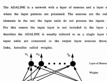
The ADALINE is a network with a layer of neurons and a layer of input units where the input patterns are presented. The neurons are the only processing elem ents in the net; the input units do not process the inputs they receive. For this reason the input layer is not included in the layer counting and therefore the ADALINE is usually referred to as a single layer network. The input units are connected to the output layer neurons through weighted links, hereafter called weights.
Layer of Neurons
Weights
Layer of Input units m
I I I
figure 2.1 - The architecture of the ADALINE network
[image:33.612.81.494.115.427.2]Chapter 2. An Introduction to A rtificial N eural Nets
W
figure 2.2 - The ADALINE network with a single neuron.
An input to the network in figure 2.2 is a vector
7 = (2.1.1)
where /^ .../^ are real values. There is an extra input in the input layer, Iq,
usually referred to as the bias. The weight linking this extra input to the neuron acts as the adjustable threshold in the Perceptron networks. The extra input is constantly set to 1.
As a m atter o f notation a pattern is defined in here has having two components: the input vector as defined in (2.1.1), also referred to as the input pattern, and the targets or desired outputs.
The functioning of the net is very simple, the input pattern is presented at the input units, collected by the weights and sent to the neuron. An excitation which is a weighted sum of the inputs present in the input pattern is com puted, and afterw ards a function, usually referred to as activation function, is applied to this value to produce an output.
n
ex= ^ /y Wy (2.1.2)
j = 0
w here Ij is the com ponent o f the input vector and w j is the weight connecting the input unit j to the neuron. The index j starts at 0 to include the bias input, usually set to 1 as mentioned before. The index n is the number o f components of the input pattern.
The activation function / of a neuron, when used for learning in the ADALINE proposed by Widrow and Hoff (1960) is a linear function. Once the network has learned and is put to use, the activation function can be replaced by a threshold function if the problem is a classification one. However, during training the activation function selected must be differentiable.
The output can be for example computed as
O = f (ex ) = ex (2.1.3)
where ex is as defined in (2.1.2) and O is the output.
Once the output is computed for an input pattern one can compare it with a target output for the respective pattern. If the output obtained is equal to the target output then nothing is done. Otherwise the weights m ust be adjusted so that a correct output is obtained.
The error for a pattern can be defined as
£ = ^ ( 0 - r ) 2 (2.1.4)
Chapter 2. An Introduction to A rtificial N eural Nets
If one considers a net with m neurons in the output layer then the total error b eco m es
= - r p 2 (2,1.5)
J
where O j is the output obtained at output unit j and Tj is the target for output
unit j.
The delta rule presents a way to change the w eights so that the error decreases. The more general form ula for the error presented in (2.1.5) is used here to describe the learning rule. The delta rule uses gradient descent to update the weights after each pattern has been presented to the network and its error computed.
The weights are updated according to
(2.1.6)
where w (j is the weight connecting from input unit i to neuron j and q is a
real constant called learning rate. To com pute the derivative present in (2.1.6) the definition of TE in equation (2.1.5) is used:
oflE
^ (2.1.7)
The derivative in the right side of (2.1.7) can be easily computed using the definition of O in (2.1.3), and (2.1.2).
dOj
dwtj — h (2 . 1 .8)
So, collecting the results from (2.1.6) to (2.1.8), the weight update form ula b eco m es
2.1.1. A graphical perspective of the ADALINE
Each input pattern can be represented as a point in Euclidean space. This space has as many dim ensions as the number of input com ponents of the pattern. For instance, let us consider a simple problem, the logical AND, with two inputs. A classification problem is selected for this section since the ADALINE was initially conceived as 'an adaptive pattern classifier' (Widrow and H off 1960). For sim plicity reasons and without loss the targets presented in the example are -1 and 1 instead of 0 and 1 as in the real logical AND p ro b le m .
The set of patterns contains four patterns, each has two inputs and a target as described in table 2.1.
Input 1 Input 2 T a rg et
0 0 -1
0 1 -1
1 0 -1
1 1 1
Table 2.1 - logical AND patterns
Chapter 2. An Introduction to A rtificial N eural Nets
(1,0)
(1,1)
(0.1) I
(0,0)
figure 2.3 - The logical AND patterns represented in input space. The black spot indicates that the target is 1, the target is -1 fo r the rem aining patterns.
Since the logical AND is a classification problem there is no need to actually achieve targets of 1 and -1 since what is required is only to separate the outputs for the patterns in one class from the outputs obtained for the patterns in the other class. In the general case, using binary output values of -1 and +1, a pattern is considered to be correctly classified if the pattern's output sign is equal to the sign of the target for the respective pattern.
For a particular w eight state there is an input space region in which the patterns will have negative inputs and an input space region where the patterns will have a positive output. Between these two regions are the points which have a 0 output. These latter points obey the following equation,
n
2,Wy/; = 0
(2.1.10)
j = 0
w here w j is the weight state connecting the input unit to the output neuron, Ij is the component of the input pattern, and n is the total number
Equation (2.1.10) can be reform ulated, by separating the bias from the other inputs, as
n
'Y .ljV /j = -wo (2.1.11)
j = 1
where is the bias weight. The value Iq , being the bias, is a constant value
set to 1 as mentioned before in §2.1 and therefore it has been omitted from the e q u a tio n .
This equation, (2.1.11), defines a hyperplane in input space. Patterns to one side of the hyperplane have negative outputs while patterns to the other side of the hyperplane have positive outputs. If the bias term was absent from (2.1.10) then the hyperplane would have to go through the origin of the input space and the logical AND problem would be unsolvable using the ADALINE.
Chapter 2, An Introduction to A rtificial N eural Nets
(1,0)
(1,1)
(0,1) ^
(0,0)
figure 2.4 - A hyperplane dividing the input space.
In this case it is possible to divide the input space in two regions in such a way that in each side of the hyperplane only patterns of the same class are to be found. When such a situation occurs the problem is said to be linearly separable. Both ADALINE and the Perceptron are limited in only being able to solve linearly separable problem s. There are though, many problem s which are not linearly separable. The logical exclusive-OR, for example, is not a linearly separable problem and therefore can not be solved by either ADALINE or the Perceptron. For a more detailed analysis of the logical exclusive-OR problem refer to §2.2.3.
2.1.2. Conclusion
The ADALINE network is a very simple learning device which was invented originally for pattern classification. It can learn to perform all classification
tasks where the property of linear separability is present.
2.2.
M ultilayer Feedforw ard Networks
2.2.1. Architecture Definition
As m entioned before, a single layer netw ork is only capable o f solving linearly separable problem s. This m akes this device a very lim ited one, sim ple problem s like the logical exclusive-O R cannot be solved using the ADALINE.
If, however, one could use more than one neuron to partition the input space and com bine these partitions for input into other neurons then m ore complex problems could be solved.
N eurons organised in this way are said to form a m ultilayer perceptron netw ork or m ultilayer feedforw ard network. The term feedforw ard is used because the signal is propagated from the input layer to the output layer w ithout recurrent connections, i.e. connections that form cyclic paths in the network. As a matter of notation, an index is attributed to each layer relative to its position in the network, for instance the input layer is layer 0, the output layer has an index n where n is the total of layers excluding the input layer. In this thesis, it is further assumed that, unless specifically stated otherwise, a unit in layer i connects to all the units in layer i+1 and only to these units.
Chapter 2. An Introduction to A rtificial N eural Nets
The layers between the input units and the output layer are called hidden layers. A network can have as many hidden layers as desired.
Outputs
Output Layer
weights
Hidden Layer
weights
Input Layer
Inputs
figure 2.5 - An example o f a multilayer feedforward network.
In figure 2.5 an example of a m ultilayer feedforward network with a single hidden layer is presented. Notice that in figure 2.5 the bias unit is not present. This unit must be added as an extra input, set permanently to 1, and is linked to all neurons in the hidden and output layers.
2.2.2. F eeding a P a tte rn to the N et
In this section the formulas to compute the output of a pattern based on its inputs are presented. Initially a description of a neuron is presented to introduce the form ulas needed.
A neuron in a m ultilayer feedforw ard network is sim ilar to the ADALINE neuron, the only difference being in the activation function. Rum elhart, Hinton and McClelland (in Rumelhart, McClelland et. al., 1986) explain why a linear activation function for the hidden units will provide no advantage to m ultilayer feedforward networks when compared with the ADALINE network.
If a m ultilayer feedforw ard netw ork uses linear activation functions then a solution weight state would satisfy the following equation:
T = * W2 * ... * W„) (2.2.1)
where T is a matrix with rows ti that stand for the target values for pattern i, I is a m atrix where each row is an input pattern, and W j is the matrix of w eights connecting from layer j-1 to layer j. The com ponents f r o m m atrix W j are the weights connecting from neuron i in layer j-1 to neuron k in layer j. The matrix W j has k rows where k is the number of input units, the matrix has j columns where j is the number of output units.
Equation (2.2.1) can be transform ed into
0 = 1* W (2.2.2)
w h e r e
W = W j * W 2 * . . . * W „ (2.2.3)
Since matrix W j has k rows and the matrix has j columns, the matrix W
C hapter 2. An Introduction to A rtificial N eural Nets
If a solution exists for (2.2.1) then a solution exists for (2.2.2). However the m atrix W in equation (2.2.2) can be seen as the weight m atrix for a single layer network with k input units and j neurons in the output layer. Therefore if there is a solution for a m ultilayer feedforw ard netw ork w ith linear activation functions then a solution exists for a network with a single layer with the same number of input and output units. But if a solution exists for a single layer netw ork then the problem m ust be linearly separable and therefore the capabilities of m ultilayer feedforw ard netw orks using linear activation functions would be restricted to linearly separable problem s.
To circum vent this problem , Rum elhart, Hinton and W illiam s (in Rum elhart, M cClelland et. al. 1986) use instead a differentiable sem ilinear activation function for the neurons in the hidden layer and output layer. For the input units a linear activation function is used, see equation (2.1.3).
The excitation of a neuron is computed as in the ADALINE using equation (2.1.2). The activation function proposed by Rum elhart, Hinton and W illiams (in Rumelhart, McClelland et. al., 1986) to compute the output of a neuron is
= r 7 7 ' - ë x (2.2.4)
where ex is the excitation of the neuron as defined in (2.1.2).
This function represents a sigmoid which produces outputs in the range [0,1] as shown in figure 2.6.
, 10
Ouput axis
0.5
Excitation axis 0.0
-OO +00
Up to this point in this section the formulas to compute the output of a neuron were presented. From this point forward the process of computing the net's output for a given input pattern is presented.
To compute the output of a net when an input pattern is fed in, it is necessary to propagate the input signal throughout the net, layer by layer starting from the input layer. To compute the output of a neuron it is necessary to compute its excitation first. The excitation of a neuron depends on the outputs of the neurons in the previous layer which are connected to it. It is therefore necessary, in order to compute the outputs of the neurons in layer i, to have the outputs from neurons in layer i-\ previously computed. To com pute the net's output, i.e. the outputs of the neurons in the output layer, one has to com pute first the outputs for the neurons in layer 1, then the outputs for neurons in layer 2, and so on until the output layer is reached.
For instance, in a single hidden layer net like the one in figure 2.5, one has first to compute the outputs of the hidden layer neurons. Only afterwards can the outputs of the neurons in the output layer be computed.
2 .2 .3 . A G ra p h ic a l P e rsp e c tiv e fo r M u ltila y e r F e e d fo rw a rd N ets
In §2.1.1 it is shown how the ADALINE network solves a linear separable problem , in this section two examples of classification problem s which are not linearly separable are presented. These examples will be shown within the context of a general graphical perspective.
First let us analyse the case where the hidden units have threshold output functions. The threshold function used is defined in the following equation.
f(ex) = 0 if ex < 0
Chapter 2. An Introduction to Artificial Neural Nets
where ex stands for excitation as defined in (2.1.2).
In §2.1.1 it was m entioned that for the ADALINE netw ork achieving separation in a problem , i.e. obtaining the desired outputs for all patterns, was equivalent to find a complete partition of input space, i.e. a partition, in which in each of the regions there were only patterns from one class. In this section the relation betw een separation and complete partitioning is analysed for m ultilayer feedforw ard netw orks.
The logical exclusive-OR problem is a natural first choice since it is widely known throughout the com m unity as being one o f the sim plest linearly inseparable problem s. The set of patterns for the logical exclusive-O R problem contains four patterns, where each has two inputs and a target as described in table 2.2.
P a tte r n Input 1 Input 2 l a r g e t ....
1 0 0 0
2 0 1 1
3 1 0 1
4 1 1 0
Table 2.2 - logical exclusive-OR patterns
As in the ADALINE case, each pattern can be seen as a point in input space. This set of patterns can be represented graphically as in figure 2.7.
(1,0)
O
(1.1)o
(0,1) I(0,0) ^2
figure 2.7 - logical exclusive-OR patterns in input space. Black points refer to targets o f 1, otherwise the target is 0
A network with a single hidden layer is now considered to solve this problem. The netw ork m ust contain two inputs and an output neuron since that is directly defined by the problem . The m ain problem here is finding a sufficient number of hidden neurons to solve the problem.
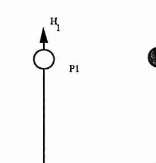
The weights connecting to each neuron in the hidden layer, called a hidden neuron hereafter, define a hyperplane in input space as in the ADALINE case. The set of those hyperplanes, one for each hidden neuron, defines a partition of the input space.
Chapter 2. An Introduction to A rtificial N eural Nets
P4
P2
H2
HI
figure 2.8 - A complete partition o f input space fo r the exclusive-OR
problem. The labels on the hyperplanes indicate which hidden neuron
they refer to. The plus and minus signs close to the hyperplanes
indicate if the output is 1 or 0 fo r the respective hidden unit fo r
patterns on either side o f the hyperplane. These signs play no part in
the determination o f a complete partition.
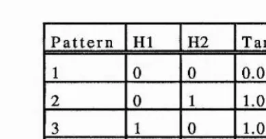
For the partition in figure 2.8 the following set of outputs are obtained for the hidden units with threshold functions.
P a tte r n H I H2 T a rg e t
1 1 0 0.0
2 1 1 1.0
3 1 1 1.0
4 0 1 0.0
Table 2.3 - Outputs fo r the hidden units using threshold futiction
[image:48.612.182.401.64.268.2] [image:48.612.195.378.503.604.2]This is because the problem presented to the output neuron is linearly s e p a ra b le .
P2
P4
figure 2.9 ~ Graphical representation o f figure 2.3
However, in contrast with the ADALINE case, achieving a complete partition does not imply being able to solve the problem. For instance let us look at the partition on figure 2.10. In this case a com plete partition is also present however separation is not possible.
H2
+
O "
+
P l (
J
—HI
P2
figure 2.10 - A complete partition fo r the XOR problem
[image:49.612.206.360.109.270.2]C hapter 2. An Introduction to A rtificial Neural Nets
P a tte r n HI H2 T a rg et
1 0 0 0.0
2 0 1 1.0
3 1 0 1.0
4 1 1 0.0
Table 2.4 - Outputs fo r the hidden units using threshold function base on figure 2.10.
If one compares the outputs from the hidden units with threshold function in figure 2.10 with the inputs of the training set on table 2.2 one can see that the hidden units are doing nothing to solve the problem which rem ains that of XOR. The outputs from the hidden units with threshold functions are still not lin early separable.
A com plete partition through the hidden layer is therefore not sufficient to achieve separation on the output unit.
Is com plete partitioning necessary for achieving separation on the output unit? The answer is affirm ative, see Nilsson (1965). Assume an incom plete partition, i.e. a partition so that in at least one of the regions there are patterns from both classes. This im plies that there will be patterns from different classes with the same hidden unit outputs because all patterns in a region have the same hidden unit outputs and there is at least one region with patterns from different classes. As far as the output unit is concerned there is no difference betw een patterns in the same region. Therefore a correct classification for all patterns in the training set is im possible without a com plete partition.
[image:50.612.193.388.81.183.2]hidden neurons. It is however a necessary condition to achieve separation as shown above.
There is however a theorem by Nilsson (1965) that relates more strongly hyperplane partitioning to separation:
Given P hyperplanes w hich form a nonredundant^ partition of two classes with a finite number of elements, if exactly P+l cells^ formed by the partition are occupied by patterns then the problem is solvable with a single hidden layer architecture using P hidden neurons.
Going back to the XOR problem we can see that the input space partition in figure 2.8 satisfies the theorem conditions because :
• P = 2, i.e. there are 2 hyperplanes and 3 regions occupied;
• The partition is nonredundant, i.e. it is impossible to remove a hyperplane without having patterns from both classes in the same region;
• The training set is finite.
Therefore, and based only on the theorem, it is possible to conclude that the XOR problem is solvable with a single hidden layer feedforw ard architecture with two threshold hidden neurons. The above theorem provides a useful visual way to check if a certain partition can provide separation with single hidden layer feedforward networks before training in 2-D.
1 A nonredundant partition is a com plete partition with the property that if any one of the separating hyperplanes is removed, at least two nonempty regions will merge into one region
Chapter 2. An Introduction to A rtificial Neural Nets
Another example, the chequerboard problem, Weir, Lansley and Clark (1993), is now presented to show a need for using more than one hidden layer. Notice that this problem has an infinite set of patterns, the finite version of the problem will be dealt with later in this section.
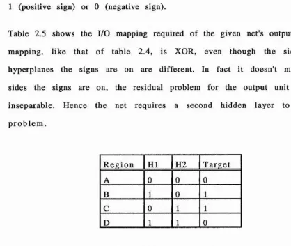
The desired input space classification for the chequerboard problem is presented in figure 2.11. Assume that the net used to try to solve the problem is a single hidden layer net with two threshold hidden neurons. Furthermore, assume that the threshold hidden neurons produce the hyperplanes labelled in the figure as HI and H2, and that the signs presented for each hyperplane indicate if the output is 1 (positive sign) or 0 (negative sign).
HI
+
-A
-f I
D
h:
fig u re 2.11 - A 2-D input space with a chequerboard desired
classification. The darker areas represent desired targets o f 0 and the
lighter ones desired targets o f 1. The labels A through D indicate
regions o f input space. The hyperplanes selected produce a complete