Don’t look down: the consequences of job loss in
a flexible labour market
∗Richard Upward†
University of Nottingham
Peter Wright
University of Sheffield
Accepted by Economica August 2017
Abstract
We estimate the earnings, hours and income effects of job loss for a representative
sample of UK workers from 1991–2007. We follow workers before and after job loss,
regardless of their labour market state, and we match displaced workers with similar
non-displaced workers. This provides a more comprehensive picture of the effect of
job loss in the UK than previously available. Job loss causes a long-run reduction in
income which is mainly due to reductions in monthly pay rather than in employment
propensity. Income from other labour market states and from welfare payments does
little to compensate for income losses. This lack of a “safety net” means that job loss
in the UK has a similar impact to job loss in the US.
JEL codes: J65, J63, C21.
Keywords: Job loss, displacement, unemployment, unemployment insurance.
∗
The authors would like to thank the participants at the OECD conference on worker displacement held in Paris in May 2013, the annual WPEG conference in July 2013, the CESifo area conference on employment and social protection in May 2014, the 26th annual EALE conference in September 2014, the IWH workshop on firm exit and job displacement in July 2015 and two anonymous referees. The data used in this paper are available from the UK data archive study number 5151. All programs used for data
preparation and results are available fromhttp://www.nottingham.ac.uk/~lezru
†
Corresponding author: emailrichard.upward@nottingham.ac.uk
1
Introduction
Every year in the UK, one in every four workers will end their current employment spell, and one in every six of these will do so because they lose their job.1 Evidence shows that job loss, or displacement, has a large and persistent impact on workers’ earnings and well-being in general.2 Quantifying the size of these losses, and understanding how workers respond to displacement is therefore important from the perspective of policy-makers wishing to ameliorate its impact. However, systematic evidence for the UK is surprisingly limited. We therefore provide new and more comprehensive evidence of the costs of displacement in the UK. We follow workers for up to a decade after displacement across all subsequent labour market states and therefore track all individual sources of income, including welfare payments. Earlier studies have typically considered these aspects in isolation; we provide a unified treatment. We show that the patterns of wage and employment loss are more similar to those in the US compared to those in other European countries. Displaced workers in the UK typically do not remain unemployed for long, but if they re-enter employment it is in lower-paying jobs. Income from alternative sources, such as self-employment and welfare benefits, does little to compensate displaced workers.
The existing literature on the effects of displacement typically finds that there are very large short-term consequences on employment and earnings, and that earnings losses persist for many years. Studies for the US include Ruhm (1991), Jacobson et al. (1993) (henceforth JLS) and more recently Couch and Placzek (2010) and Davis and von Wachter (2011). Since JLS, it has become increasingly common to rely on administrative data, such as social security earnings records, to estimate the cost of displacement. These data offer several advantages. They provide an externally validated measure of displacement based on plant closure or large employment reductions, accurate measures of earnings, and large samples. However, administrative data are often silent on what happens to displaced workers who leave employment and enter other labour market states such as self-employment, training or early retirement. Administrative data also often contain little demographic information which would allow the construction of suitable counterfactuals.
11991–2008, BHPS. See Table1. 2
Finally, administrative data rarely contain information on working time, which means that one cannot determine whether falls in pay are caused by reductions in hours or wages.
It remains the case that very little is known about the effects of job displacement in the UK. Administrative data (such as social security records) are not currently available to researchers in the UK. The only existing estimates of the earnings losses of displacement come from Borland et al. (2002), who use household survey data from the early 1990s and Hijzen et al. (2010), who use employer survey data matched to firm registers for the period 1994–2003.3 The UK is an interesting test-case for the study of displacement because it has one of the lowest levels of employment protection in the OECD,4 and also offers very low state benefits for unemployed workers.5 An important issue then is whether these institutional features lead to similar post-displacement earnings and income patterns to other “flexible” labour markets such as the US.
In this paper we use household survey data, which offers a number of advantages over the available administrative datasets. First, we can follow individuals through all labour market states before and after displacement. This means that we do not need to exclude individuals from the analysis who subsequently have zero earnings from employment.6 Second, we have information on income from all sources, including welfare payments and earnings from self-employment. This allows us to directly assess the extent to which alternative sources of income and the welfare system compensate for lost earnings. Third, survey data from a long panel allows us to use a much richer set of pre-displacement characteristics with which we can match displaced and non-displaced workers. Finally, we are able to decompose changes in pay into changes in wages and hours of work. In contrast to the earlier work using survey data for the UK (Borland et al., 2002), we are able to follow a larger sample of displaced workers over a much longer period of time. Our methods allow us to measure earnings loss at various points in time after displacement, and also allow us to follow workers regardless of their subsequent labour market state.7 In 3Doiron and Mendolia (2011) use the same survey data as in our paper to study the effects of
displace-ment on divorce, which we discuss in more detail in Section2.
4See Venn (2009), which ranks the UK 38th out of 40 for the extent of employment protection.
5
OECD measures from http://www.oecd.org/els/benefitsandwagesstatistics.htm show that the
UK has the least generous net replacement rates for the initial phase of unemployment in the OECD. 6
This is a common restriction used by those with social security earnings data. 7
Borland et al. (2002) only compare earnings for those workers who return to employment after dis-placement. By definition, this is a selected sample of displaced workers.
addition, we explicitly construct matched treatment and control groups and use methods which allow us to directly compare our results with those from other countries.
However, the use of survey data also has some limitations. First, our measure of displacement is self-reported rather than inferred from plant closure or employment re-ductions. It therefore seems possible that some of the displacements we observe are not the result of job destruction which is exogenous to the individual. To mitigate this, we compare displaced workers to non-displaced workers who have observably similar pre-displacement characteristics and labour market outcomes, and we allow for selection on unobserved fixed characteristics. We also compare workers who report “redundancy” as opposed to “dismissal”. Second, self-reported displacements may suffer from recall bias (for example, respondents may be more likely to accurately recall more costly events). To mitigate this possibility, we consider only recall information from the previous 12 months. Finally, our survey data has smaller sample sizes which limit the extent to which we can reliably estimate the impact of displacement on narrowly defined sub-groups.
We show that job displacement in the UK causes an immediate loss in income of nearly 40%, and a long-run reduction in income of approximately 10%. These estimates are similar to the only comparable results for the UK (Hijzen et al., 2010). However, the estimated composition of the loss is different. Hijzen et al. found that the majority of earnings loss is accounted for by lower employment rates rather than lower earnings. In contrast, the results in this paper show that the majority of the long-run loss (80%) is accounted for by a reduction in post-displacement earnings rather than lower employment rates. This suggests that the consequences of displacement in the UK are very similar to the US. Couch and Placzek (2010), who use a comparable methodology, find imme-diate losses of 32% and long-run losses of 12%. Our results are also consistent with the large US literature which uses survey data, and which therefore relies on self-reported displacement.8
We do find a small long-run reduction in the probability of employment, because some displaced workers enter a variety of other labour market states, namely long-term unemployment, self-employment, sickness or disability and early retirement. However,
income from these sources does little to compensate the income losses following displace-ment. Total income from other sources, including self-employment income, unemployment insurance, retirement income and invalidity benefit reduce losses by only 15% in the first 12 months after displacement, and by about 12% after 10 years.
The paper is structured as follows. In Section 2we explain how our paper relates to the existing literature on job displacement. In Section3 we describe the data that we use and how we construct a measure of displacement. Section 4 explains our basic method, which is a variant of a standard difference-in-difference model. In Section5 we illustrate the basic patterns in the data and in Section 6 we report the effects of displacement on earnings and non-labour income as well as hours of work. Section7concludes and discusses our findings in the context of the “flexibility” of the UK labour market.
2
Literature review
This paper relates to three main areas of the literature that examine the impact of job displacement. The first is the long run impact on employment and earnings. The seminal article is JLS, who use administrative data for Pennsylvania between 1980 and 1986 to ex-amine the earnings losses of high seniority men who separate from plants which experience large (>30%) employment falls. They find that even six years after the event, earnings losses remain at 25% compared to pre-displacement levels. These contrast with somewhat smaller estimates using survey data such as the Panel Study of Income Dynamics (Stevens, 1997) and the Displaced Worker Survey (Farber, 1997). Couch and Placzek (2010) argue that these very large estimated losses are primarily due to the fact that JLS examine a period of particularly high displacement among manufacturing workers in a heavily in-dustrialised state. To demonstrate this, Couch and Placzek use similar data, but examine Connecticut from 1993–2004. Although immediate losses remain high at 32–33%, the es-timates of long run losses are reduced to 13–15% after six years.9 These are in the range of earlier estimates. They are also remarkably consistent with the analysis of Morissette 9Couch et al. (2011) retain the assumption found in Jacobson et al. (1993) that individuals must have
positive earnings in every year post displacement. When they drop this assumption losses rise by 15-18%: See footnote 14.
et al. (2013) for Canada. For the UK, Hijzen et al. (2010), using employer survey data matched to firm registers, also find large and persistent effects. In the first five years, losses from firm closure are in the range 18–35% and for mass layoffs 14–25%. However, in contrast to the US literature, Hijzen et al. (2010) argue that these are substantially the result of the high and persistent non-employment rates of the displaced rather than lower earnings on return to work. Couch and Placzek (2010) emphasise the potential impor-tance of the use of matching estimators to control for systematic selection in those who are displaced, although they find only weak evidence for an overstatement of the estimated impact of displacement without matching, perhaps because they have a limited number of demographic variables available for matching.
The second related area concerns the impact of welfare payments on the earnings losses of the displaced and whether this can lead to systematic differences between coun-tries.10 Welfare payments can provide temporary compensation for short-term earnings losses, but may also prolong search. Increased search duration has two countervailing effects on earnings losses because as well as extending periods out of work, it may also lead to higher post-displacement wages.11
Schmieder et al. (2010) use administrative data to examine mass layoffs in West Germany in 1982. Those displaced from stable jobs have long term earnings losses of 10– 15%. This is mainly due to a decline in post-displacement wages, as in the US. Schmieder et al. note that although they are examining displacement in a recession year, which may lead to larger losses, they argue that earlier studies using survey data which find smaller losses for Germany (e.g. Burda and Mertens, 2001) include workers subject to temporary layoffs whose losses are likely to much lower. They also show that, even in a country such as Germany with a relatively generous welfare system, the payments only compensate for a small fraction of the earnings losses and only in the immediate aftermath of displacement.
Ehlert (2012) examines the role that welfare benefits play in moderating the impact of transitions from work to unemployment using survey data in both the US and Germany.
10
See OECD (2013) for a summary table of other studies. 11
The methodology makes it difficult to make direct comparisons because the sample includes both voluntary and involuntary job separations. Nevertheless, Ehlert does find similar post-displacement trajectories for displaced workers in both countries.12 However, men in
the US rely relatively more on family resources to buffer their income compared to men in Germany, who rely more heavily on the welfare state. Womens’ income losses are mainly compensated by higher partner earnings in both countries. Single individuals suffer in the US in particular, as they lack both state and family support.
Nordic countries are regarded as having the most comprehensive social safety nets. Eliason (2011) examines the long-run effects of plant closures, and the potentially miti-gating impact of social insurance using longitudinal data for Sweden. He finds significant and long-lasting impacts of displacement on the earnings of married males, but somewhat smaller than that found for the US.13 Average annual losses are approximately 6% 4–12 years after plant closure. Eliason finds a big initial uptake in unemployment insurance, but only limited impacts on sickness/disability insurance or other means tested benefits.
Hardoy and Schøne (2014) look at the role that the welfare state plays in mitigating income losses from displacement in 2002 using register data for Norway. The authors also account for family effects and tax payments. They find that annual earnings decline by only approximately 5% after displacement and, although they only have three post-displacement years, argue this effect is persistent.14 Norway has a particularly generous
welfare system in comparison to most countries and 15–20% of short term losses are compensated by unemployment benefits. However, once health-related benefits, public transfers and changes to tax are accounted for, the negative impact on the household is reduced by 65%.
The third area to which our paper relates is whether displacement leads to entry into other labour market states, such as self-employment or early retirement. For example, Farber (1999) uses the Displaced Workers Survey (DWS) for 1994 and 1996 and examines the status of individuals a year after displacement. He finds high entry rates of
dis-12
Comparisons with other studies are also hindered because Ehlert considers household income of married couples rather than individual income.
13
No effect is found for married women. 14
This result is comparable to that of Huttunen et al. (2011), who estimate an initial loss of 4.8%, which remains at 3% after seven years.
placed workers into alternative work arrangements as a temporary state before re-entering employment. Von Greiff (2009) estimates that displacement doubles the probability of entering self-employment within one year of the displacement. Fairlie and Krashinsky (2012) examine business creation using the PSID and CPS. Although the focus is on liq-uidity constraints, they analyse data separately for job losers and non-job losers. The find high entry rates into self-employment from wealthy elderly job losers who have both the necessary capital and relatively poor alternative employment prospects. Such an effect is also found by Nykvist (2008) using register-based data for Sweden. Examining the im-pact of plant closures in 1987 and 1988 she finds that displacement almost doubles the likelihood of entry into self-employment and those in worse labour market positions react more strongly.15
Turning to the impact on retirement, Chan and Stevens (1999, 2001) find, for the US, that men who are displaced postpone retirement in an attempt to rebuild savings. Tatsiramos (2010), using household survey data on 45-64 year olds from the European Community Household Panel from Germany, Italy, the UK and Spain, finds that individ-uals in those countries which offer relatively generous unemployment benefits and early retirement provisions are less likely to return to work before 60 and more likely to retire post 60. For Norway, Huttunen et al. (2011) find that the most important impact of dis-placement is not in terms of reduced earnings, but in terms of the probability of movement out of the labour force due to the generosity of early retirement schemes and disability pensions.
In this paper we provide the first comprehensive evidence of the costs of job displace-ment in the UK which takes into account all three of these aspects. We consider short- and long-term losses; we consider the effect of welfare payments; and we consider the effect of transitions into other labour market states. Further, we are able to precisely match displaced workers with a comparable control group thanks to detailed pre-displacement characteristics.
15
3
The data
The British Household Panel Survey (BHPS) is an annual survey of about 5,500 households recruited in 1991, containing approximately 10,000 interviewed individuals. The sample is intended to be nationally representative. Adults in the sample are re-interviewed annually; children are interviewed when they reach the age of 16. Individuals in the sample are followed regardless of whether they remain in the same household or join new households. The BHPS continued until 2008, when it was replaced by and incorporated into the UK Household Longitudinal Survey (HLS).16
We use data from all BHPS waves 1–18, interviews for which took place from 1991 to 2009. After appending all 18 waves, the data contain 32,379 individuals and 238,992 person-years. We use all members of the original sample who have full interview outcomes, which results in a sample containing 29,264 individuals and 219,592 person-years. The data are an (approximately) annual panel. For each individual we observe a sequence of interviews from waves 1991 to 2009.17 The median duration between interviews is almost exactly one year, and 90% of interviews take place within 400 days of the previous interview. Each respondent is asked to report their current labour market status at the time of the interview. In addition, they are asked for information on any labour market spells which began after the 1st September in the previous year, including start and end dates and the reasons why jobs ended.
Using the recall information from the following year’s interview, we calculate when the spell in progress at the date of interview ended, and the reason why it ended.18 In our basic specification, displacement is defined as occurring if an employment spell ends due to “redundancy” or “dismissal” (the full list is given in Appendix A.) As noted by Borland et al. (2002), the distinction between redundancy and dismissal in the UK is
16The first interviews for the BHPS sample in the HLS did not take place until 2010 and 2011, meaning
that there is a much larger gap (median 645 days) between the final interview in the BHPS and the first interview in the HLS, during which labour market status and earnings are not recorded. We therefore use only BHPS data in this paper. A detailed description of the BHPS data can be found in Taylor et al. (2010). The HLS is described in Institute for Social and Economic Research (2011).
17The precise interview date varies over the year, although 85% of interviews take place in September,
October or November. A small number of interviews take place in the following year, hence some interviews take place in 2009.
18
The precise method for creating the link between the recall information from wavet+1 and the current information from wavetis described in detail in AppendixA.
Year Number of obs.
Number of emp. spells
Prop. emp. spells ending in displacement
Prop. emp. spells ending other reasons
Prop. emp. spells continuing
1991 8,309 4,093 0.058 0.168 0.774
1992 7,907 3,852 0.062 0.187 0.751
1993 7,873 3,782 0.050 0.197 0.753
1994 7,970 3,877 0.052 0.208 0.740
1995 8,027 3,994 0.049 0.191 0.760
1996 8,483 4,277 0.042 0.214 0.745
1997 8,164 4,230 0.047 0.224 0.729
1998 8,076 4,212 0.045 0.229 0.726
1999 9,129 4,580 0.045 0.226 0.730
2000 10,667 5,555 0.046 0.230 0.723
2001 16,142 7,867 0.042 0.194 0.764
2002 14,501 7,110 0.039 0.204 0.757
2003 14,647 7,375 0.034 0.204 0.761
2004 13,293 6,644 0.036 0.205 0.759
2005 13,371 6,669 0.036 0.156 0.808
2006 12,836 6,343 0.034 0.176 0.790
2007 12,396 6,160 0.037 0.158 0.805
2008 475 265 0.042 0.170 0.789
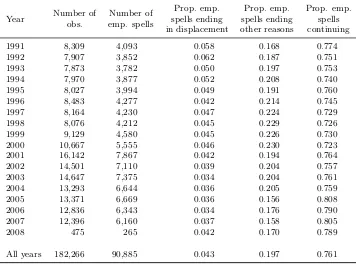
[image:10.595.119.475.86.350.2]All years 182,266 90,885 0.043 0.197 0.761
Table 1: Basic sample characteristics 1991–2008. The sample includes only those individuals who have an interview in the following wave and therefore includes only interviews from wave 1–17. Displacement in this table is defined to include redundancy, dismissal or the end of a fixed-term contract.
somewhat blurred. In particular, those answering that they were “dismissed/sacked” may include both those who were dismissed for individual reasons as well as those whose job was destroyed for external reasons. In contrast, Doiron and Mendolia (2011) argue that the distinction between these two responses is important, and that individuals who are dismissed for individual reasons may report that they were made redundant. We examine the distinction between these two responses empirically, by testing whether post-displacement behaviour is distinct.
The resulting data are described in Table 1. The proportion of employment spells observed in wavet which are still in progress in wave t+ 1 is between 70% and 80%. Of those which end, approximately 18% are classified by the respondents as “displacement” (redundancy, dismissal or temporary jobs ending). Note that the measurement of displace-ment used here will tend to be an under-estimate for short spells of employdisplace-ment, because a spell which starts after the interview in wave t and ends before the interview in wave
t+ 1 will not be recorded.
Redundancy (BHPS)
End of temp. jobs (BHPS) Dismissals
(BHPS) Redundancy
(ONS)
0.00 0.01 0.02 0.03 0.04 0.05 0.06
Probability of displacement
[image:11.595.135.460.89.309.2]1991 1992 1993 1994 1995 1996 1997 1998 1999 2000 2001 2002 2003 2004 2005 2006 2007 2008 2009 2010 2011 2012
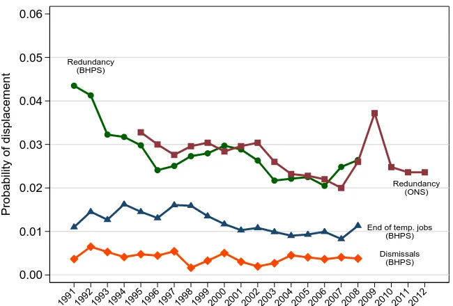
Figure 1: Estimates of probability of displacement from BHPS compared to Office for National Statistics redundancy series (Heap, 2004). The ONS series is calculated from the UK quarterly Labour Force Survey.
for National Statistics redundancy series calculated from the Labour Force Survey, shown in Figure 1.19 Both series reflect the improving labour market up until the 2008–2009 recession. The incidence of temporary jobs ending is less strongly counter-cyclical, while the dismissal rate is too small to draw conclusions.
4
Methods
We define a series of dummy variable Dci, c = 1991, . . . ,2007 which take the value 1 if individual i experiences displacement between the wave t = c and the wave t = c+ 1 interview, andDci = 0 if they do not. Those withDci = 0 will therefore include individuals who change job betweencandc+ 1 for reasons other than displacement.20 Dicis constant for each individual for a given value ofc, but each individual has a separate indicator for
19
Series BEIR, calculated as the number of respondents whether working or not working, who reported that they had been made redundant or had taken voluntary redundancy in the previous three months as a fraction of number of employees in the previous quarter. See Heap (2004) for a discussion of ONS measure of redundancy.
20Therefore we do not restrict the control group to include only those who continue in employment after
wavec. This contrasts with JLS, whose control group consists only of those whoremain in the same firm. Their definition of earnings losses is therefore “the change in expected earnings if . . . the worker would be displaced . . . rather than being able to keep his or her job indefinitely.” (Jacobson et al., 1993, p.691). Instead, our counterfactual is more general, and is intended to measure the earnings of the displaced
workers had they not been displaced. In AppendixDwe demonstrate that this restriction on the control
group has a significant impact on the estimated losses.
each cohortc. We refer to the sample with Dic= 1 as the cohort c treatment group and those withDic= 0 as the cohort ccontrol group.
To construct the data for a particular cohort, we restrict the sample to all those who are interviewed in wave c and wave c+ 1, who are in employment in wave c and aged between 20 and 60 in wavec. Note therefore that the control group for a particular cohort may include those who are in the treatment group in other cohorts. Similarly, the treatment group for a cohort may include those who are in the control group in other cohorts.
Define yit to be the outcome of interest for individual i in wave t. These outcomes include employment status (e.g. in employment, in self-employment, hours of work) and various measures of income (e.g. income from employment, self-employment, welfare pay-ments). yitis measured both beforet≤cand aftert > cthe displacement event. We wish
to estimate the impact ofDic onyit. The least restrictive method would be to estimate a
standard difference-in-difference model separately for each displacement cohort. However, we observe a relatively small number of displacements in each cohort (see Table1), and so we instead stack together cohorts and impose the restriction that the effect of displacement relative to the displacement date is the same for each cohort.21 Once stacked, each row in the data is identified byi,c and tbecause individuals may appear in several cohorts.
For those withDci = 1 we record the date on which the displacement occurred. This date is recorded to the nearest day, although since it comes from recall information in the next wave of data, it seems likely to be somewhat approximate. For those with Dic = 0 we choose a random date in between the interview in waves t and t+ 1, drawn from a uniform distribution. The difference between the interview date and the displacement (or non-displacement) date, grouped into years, is relative time, denoted rict. Thus rict = 0
in the year immediately preceding the displacement andrict = 1 in the year immediately
after. We restrict attention to−10≤rict ≤10 to ensure sufficient numbers of treated and
control observations in each year. 21
Our principle estimating equation is then
yict=αic+
10 X
r=−9
γrTtr+
10 X
r=−4
δr(TtrDic) +it. (1)
We include a person-cohort fixed effect αic which captures any pre-existing difference in yit between the treatment and control groups more than five years before displacement.
The dummy variables Ttr indicate time relative to the displacement event which occurs between r = 0 and r = 1. The coefficient δr is a difference-in-difference estimate of the effect of a displacement which occurred r years earlier. δr is estimated for five years
(r=−4,−3, . . . ,0) before displacement to allow for the possibility that displacement has
effects before the event, and for up to 10 years (r = 1,2, . . . ,10) after displacement. We allow the errorsitto be clustered byiacross cohorts. The difference-in-difference estimate
δr controls for any pre-existing difference inyit between the treatment and control groups in the base years, which are at least five years before displacement (r=−10,−9, . . . ,−5).22
We can allow for differences in pre-existing earnings trends between the treatment and control groups. JLS note that one can estimate this model by deviating each variable from the person-specific time-trend (as opposed to the person-specific mean in the FE model) and estimating by OLS. Alternatively, one can difference the data and then estimate using FE (Wooldridge, 2010, p.375).
We can also control for differences in observable characteristics between the treat-ment and control groups during the pre-displacetreat-ment period. We do this by a combination of one-to-one and propensity score matching, which ensures that we are comparing similar individuals in the treatment and control groups. We match only individuals from the same cohort. This means that individuals cannot be matched with themselves, and that indi-viduals are matched with others who face the same aggregate labour market conditions. Following Rosenbaum and Rubin (1983), define p(xi) as the probability of experiencing
displacement in the future given a vector of characteristics xi. p(xi) is estimated using
a Probit model. The matched sample then consists of displaced and non-displaced indi-viduals who have similar values of pd(xi). Once a suitably matched sample is obtained, 22Choosing a base year too close tor= 0 means that any pre-displacement dip in earnings will tend to
increase the estimate ofδr.
the average effect of displacement on the displaced can be estimated by simply comparing
yit between the (matched) treatment and control groups for any value of r. One can also use difference-in-difference models to additionally control for any level differences which remain after matching. Using survey data allows us to estimate a rich model for p(xi)
which includes detailed pre-displacement characteristics.
5
Descriptive evidence
Before providing formal estimates of the cost of displacement, in this section we the key patterns in the data. We show the extent to which displaced workers are non-randomly selected, and we show the patterns of employment, earnings and income before and after displacement.
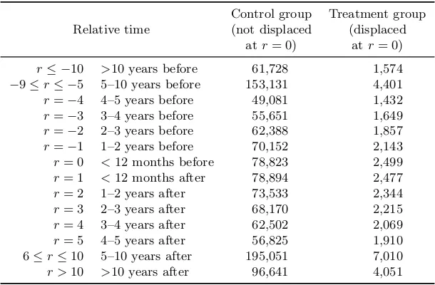
The largest sample we use comprises all individuals who are in employment, aged between 20 and 60 and who have information on the outcome of the employment spell in progress at the time of the interview. Our basic definition of displacement includes re-dundancy and dismissal, but excludes the end of temporary jobs. The resulting treatment group comprises 2,499 individuals (37,631 observations) and the control group comprises 78,823 individuals (1,162,570 observations). The sample is illustrated in Table 2. The number of observations declines as we move further away from the displacement event be-cause of the start and end of the sample period. Nevertheless, we have a reasonable sample size of displaced workers who are observed a long time before and after displacement. The former helps us to match the control and treatment group more precisely, while the latter allows us to measure long-run effects of displacement.
Relative time
Control group (not displaced
atr= 0)
Treatment group (displaced
atr= 0)
r≤ −10 >10 years before 61,728 1,574
−9≤r≤ −5 5–10 years before 153,131 4,401
r=−4 4–5 years before 49,081 1,432
r=−3 3–4 years before 55,651 1,649
r=−2 2–3 years before 62,388 1,857
r=−1 1–2 years before 70,152 2,143
r= 0 <12 months before 78,823 2,499
r= 1 <12 months after 78,894 2,477
r= 2 1–2 years after 73,533 2,344
r= 3 2–3 years after 68,170 2,215
r= 4 3–4 years after 62,502 2,069
r= 5 4–5 years after 56,825 1,910
6≤r≤10 5–10 years after 195,051 7,010
[image:15.595.145.450.84.284.2]r >10 >10 years after 96,641 4,051
Table 2: Sample sizes for treatment and control groups by relative time
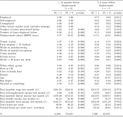
with a partner. Most of these differences between the control and treatment groups are also visible in the second column (5–6 years before displacement). In addition, workers who are going to be displaced in five years time are much more likely to be unemployed (7% compared to 3%).
The bottom panel of Table3also compares the seven outcome variables we analyse in Section6. 12 months before displacement, the treated have 5% lower wages and 6% higher hours of work, consistent with the fact that the the treated are more likely to be working full-time. Note that self-employment and benefit income are a tiny fraction of total income because the sample is restricted to be those in employment. Differences in pay and hours between the displaced and non-displaced five years before displacement are much smaller and insignificantly different from zero. There are two possible explanations for the fact that the relative earnings of the displaced workers decline prior to displacement. One is that workers who are going to be displaced experience negative shocks to their wages and job quality as they approach the point of displacement. The second is that the sample observed in employment five years before displacement is a non-random selection of those who experience displacement.
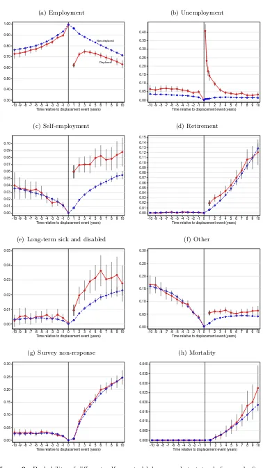
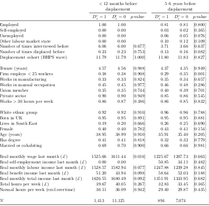
To gain an understanding of how employment patterns evolve before and after dis-placement, Figure2 illustrates the probability of observing the sample in different labour market states by relative time. Panel (a) shows that one year after displacement more than
<12 months before displacement
(r= 0)
5–6 years before displacement
r=−5
Dc
i= 1 Dic= 0 p-value Dci= 1 Dci= 0 p-value
Employed 1.00 1.00 0.77 0.80 [0.011]
Self-employed 0.00 0.00 0.03 0.03 [0.525]
Unemployed 0.00 0.00 0.07 0.03 [0.000]
Other labour market state (includes missing) 0.00 0.00 0.10 0.12 [0.086]
Number of times interviewed before 4.82 5.27 [0.000] 3.62 3.75 [0.149]
Number of times displaced before 0.20 0.11 [0.000] 0.13 0.09 [0.000]
Displacement cohort (BHPS wave) 9.17 10.01 [0.000] 11.71 12.01 [0.003]
Tenure (years) 4.27 5.10 [0.000] 4.14 4.55 [0.022]
Firm employs<25 workers 0.38 0.33 [0.000] 0.29 0.32 [0.083]
Works in manufacturing 0.33 0.18 [0.000] 0.35 0.21 [0.000]
Works in manual occupation 0.48 0.40 [0.000] 0.47 0.43 [0.005]
Union member 0.36 0.52 [0.000] 0.39 0.52 [0.000]
Private sector 0.89 0.65 [0.000] 0.86 0.66 [0.000]
Works>30 hours per week 0.85 0.80 [0.000] 0.86 0.81 [0.000]
White ethnic group 0.94 0.95 [0.055] 0.96 0.96 [0.254]
Born in UK 0.95 0.95 [0.901] 0.95 0.95 [0.983]
Lives in South East 0.23 0.22 [0.193] 0.26 0.25 [0.332]
Female 0.38 0.52 [0.000] 0.41 0.53 [0.000]
Age 38.39 39.13 [0.001] 35.46 35.57 [0.735]
Has degree 0.37 0.47 [0.000] 0.33 0.40 [0.000]
Married or cohabiting 0.70 0.75 [0.000] 0.65 0.70 [0.001]
Real monthly wage last month (£) 1481.23 1564.61 [0.001] 1213.57 1223.43 [0.772]
Real self-employment income last month (£) 0.88 6.08 [0.105] 52.93 34.67 [0.106]
Real monthly labour income last month (£) 1478.40 1553.25 [0.002] 1241.05 1249.51 [0.805]
Real benefit income last month (£) 42.23 50.36 [0.006] 57.77 55.35 [0.558]
Real monthly total income last month (£) 1562.71 1655.43 [0.000] 1342.36 1351.39 [0.792]
Total hours per week 39.94 38.22 [0.000] 32.83 32.32 [0.360]
Normal hours per week (excl. overtime) 36.19 34.25 [0.000] 29.32 28.85 [0.311]
[image:16.595.93.509.85.480.2]N 2,499 78,823 1,209 42,235
Table 3: Characteristics of displaced and non-displaced workers before displacement. Both dis-placed and non-disdis-placed groups are selected from those aged 16–60 at the time of displacement. Tenure, firm size, industry, occupation, union membership and hours per week refer only to those in employment. ‘Degree’ includes university degree, teaching qualifications and any other technical, professional or higher qualifications.
(a) Employment Displaced Non-displaced 0.30 0.40 0.50 0.60 0.70 0.80 0.90 1.00
-10 -9 -8 -7 -6 -5 -4 -3 -2 -1 0 1 2 3 4 5 6 7 8 9 10 Time relative to displacement event (years)
(b) Unemployment 0.00 0.05 0.10 0.15 0.20 0.25 0.30 0.35 0.40
-10 -9 -8 -7 -6 -5 -4 -3 -2 -1 0 1 2 3 4 5 6 7 8 9 10 Time relative to displacement event (years)
(c) Self-employment 0.00 0.01 0.02 0.03 0.04 0.05 0.06 0.07 0.08 0.09 0.10
-10 -9 -8 -7 -6 -5 -4 -3 -2 -1 0 1 2 3 4 5 6 7 8 9 10 Time relative to displacement event (years)
(d) Retirement 0.00 0.01 0.02 0.03 0.04 0.05 0.06 0.07 0.08 0.09 0.10 0.11 0.12 0.13 0.14 0.15
-10 -9 -8 -7 -6 -5 -4 -3 -2 -1 0 1 2 3 4 5 6 7 8 9 10 Time relative to displacement event (years)
(e) Long-term sick and disabled
0.00 0.01 0.02 0.03 0.04 0.05
-10 -9 -8 -7 -6 -5 -4 -3 -2 -1 0 1 2 3 4 5 6 7 8 9 10 Time relative to displacement event (years)
(f) Other 0.00 0.05 0.10 0.15 0.20 0.25 0.30
-10 -9 -8 -7 -6 -5 -4 -3 -2 -1 0 1 2 3 4 5 6 7 8 9 10 Time relative to displacement event (years)
(g) Survey non-response
0.00 0.05 0.10 0.15 0.20 0.25 0.30
-10 -9 -8 -7 -6 -5 -4 -3 -2 -1 0 1 2 3 4 5 6 7 8 9 10 Time relative to displacement event (years)
(h) Mortality 0.000 0.005 0.010 0.015 0.020 0.025 0.030 0.035 0.040
[image:17.595.112.490.76.749.2]-10 -9 -8 -7 -6 -5 -4 -3 -2 -1 0 1 2 3 4 5 6 7 8 9 10 Time relative to displacement event (years)
Figure 2: Probability of different self-reported labour market states before and after displacement 1991–2007. 95% confidence intervals around the mean based on clustered standard errors.
An advantage of the survey data, in contrast to the administrative data available for the UK, is that we can also calculate what happens to individuals who are not in employment.23 This is illustrated in the remaining panels of Figure 2. Panel (b) shows
that large increases in unemployment are short-lived. In this panel we also show estimates for three, six and nine months after displacement.24 After three months, more than 40% of displaced workers classify themselves as unemployed, but this falls rapidly to less than 15% after 12 months. After five years, unemployment rates amongst the treatment group are only slightly higher than in the control group. The pre-displacement difference in unemployment rates is also very clear from panel (b).
In panel (c) we show that displacement causes a sudden burst of entry into self-employment. After five years, 8% of displaced workers report themselves to be self-employed, compared to 4% of the control group. Panel (d) shows that displaced workers enter retirement more quickly in the first few years, but this effect is relatively short-lived.25 Panel (e) shows that displacement is also associated with higher rates of self-reported sick-ness, although small sample sizes render our estimates rather imprecise after six years. The remaining labour market states (essentially, family care and education) are shown in Panel (f).
The employment patterns shown in Panels (a)–(f) in Figure2are conditional on being interviewed: labour market status is missing for those individuals who do not participate in the survey. However, it turns out that attrition from the panel is almost identical in the treatment and control groups, shown in panel (g). The BHPS allows us to identify individuals who left the survey due to death, and this is shown in panel (h). There appears to be a small but increasing difference in mortality rates between displaced and non-displaced workers, which is consistent with the higher self-reported levels of sickness shown in panel (e), but note that the imprecision of the estimates means that we cannot reject the null of no effect on mortality.
23As noted in the literature review, administrative data for some countries (in particular Norway and
Sweden) do contain information on labour market states other than employment, and also on receipt of income from welfare payments.
24
Although the survey is annual, the fact that displacement occurs at different points within the year means that some interviews take place within three, six and nine months of the displacement date.
25
To summarise, Figure 2 shows that, 10 years after displacement, there is approxi-mately an 8 percentage point gap in employment between displaced and non-displaced workers. This gap is made up from higher rates of unemployment (2 pp), self-employment (3.3 pp), ill-health and mortality (0.5 pp), and other labour market states such as educa-tion and family care (2.2 pp).
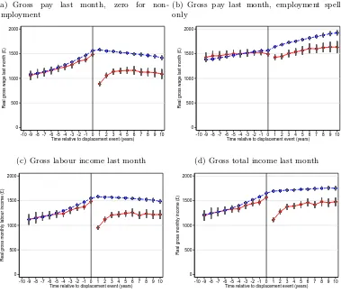
We now turn to the pattern of pay and other income following displacement. The patterns of employment in Figure2 show that alternative sources of income from unem-ployment benefit, self-emunem-ployment and retirement may reduce the costs of displacement. In contrast to administrative data, our survey data sheds some light on this issue. First, suppose that we have no information on income outside of the labour market, and we assume that indviduals not in employment have zero income. The resulting pattern of pay is shown in panel (a) of Figure3. One can see that pay losses mimic very closely the pattern of employment shown in panel (a) of Figure 2. After 10 years, pay per month in the treatment group is£330 or 23% lower than in the control group.
If we examine only those in employment then we can estimate the loss which occurs as a result of lower monthly pay in subsequent jobs, rather than the total loss (which includes periods of zero earnings). The resulting estimates are shown in Panel (b) of Figure3. In this case after 10 years the earnings gap is£289 per month or 15%. In other words, of the total 23% gap in earnings, about two-thirds is accounted for by a monthly earnings gap for those in employment, and the remaining one-third by an employment gap. A couple of other features are interesting. First, note that there is some indication of different pay growth rates before displacement, although the effects are not large. Second, there is little indication of any narrowing of the pay loss even after 10 years; if anything the pay gap gets bigger.
In Panel (c) we measure total monthly labour income, which includes any earnings from self-employment which occur after displacement. Differences between (c) and (a) are very minor because self-employment income is relatively unimportant. Note that from Figure2we know that by year 10 about 7% of the treatment group are in self-employment compared to 4% of the control group, and including self-employment earnings reduces the earnings gap from 23% to 18%. In Panel (d) we include gross monthly income from all
(a) Gross pay last month, zero for non-employment
0 500 1000 1500 2000
Real gross wage last month (£)
-10 -9 -8 -7 -6 -5 -4 -3 -2 -1 0 1 2 3 4 5 6 7 8 9 10 Time relative to displacement event (years)
(b) Gross pay last month, employment spells only
0 500 1000 1500 2000
Real gross wage last month (£)
-10 -9 -8 -7 -6 -5 -4 -3 -2 -1 0 1 2 3 4 5 6 7 8 9 10 Time relative to displacement event (years)
(c) Gross labour income last month
0 500 1000 1500 2000
Real gross monthly labour income (£)
-10 -9 -8 -7 -6 -5 -4 -3 -2 -1 0 1 2 3 4 5 6 7 8 9 10 Time relative to displacement event (years)
(d) Gross total income last month
0 500 1000 1500 2000
Real gross monthly income (£)
[image:20.595.108.487.89.414.2]-10 -9 -8 -7 -6 -5 -4 -3 -2 -1 0 1 2 3 4 5 6 7 8 9 10 Time relative to displacement event (years)
Figure 3: Individual gross income by treatment and control groups. Relative time is grouped into annual intervals. In the first panel, pay is zero for all non-employment spells. The second panel uses only spells of employment. 95% confidence intervals around the mean based on clustered standard errors.
sources, which includes benefit and pension payments. This only has a minor effect on income, reducing the gap after 10 years from 18% to 16%.
6
Results
pre-(1) Pay last
month
(2) Pay last month, emp.
spells only
(3) Self-emp income last
month
(4) Total labour
income last month
(5) Benefit income
last month
(6) Total income
last month
3–5 years before −0.009 −0.013 −0.011 −0.016 −0.002 −0.015 (0.015) (0.014) (0.008) (0.018) (0.002) (0.017) 1–3 years before −0.025 −0.034∗∗ −0.013 −0.044∗∗ −0.006∗∗ −0.043∗∗
(0.018) (0.017) (0.008) (0.019) (0.003) (0.018) <1 year before −0.037∗ −0.056∗∗∗ −0.008 −0.046∗∗ −0.005 −0.044∗∗
(0.020) (0.019) (0.008) (0.020) (0.003) (0.020) <1 year after −0.382∗∗∗ −0.151∗∗∗ 0.021∗∗ −0.366∗∗∗ 0.011∗∗∗ −0.330∗∗∗
(0.027) (0.026) (0.010) (0.025) (0.003) (0.024) 1–3 years after −0.259∗∗∗ −0.180∗∗∗ 0.016 −0.250∗∗∗ 0.005 −0.224∗∗∗
(0.025) (0.023) (0.011) (0.026) (0.004) (0.024) 3–5 years after −0.219∗∗∗ −0.156∗∗∗ 0.008 −0.223∗∗∗ −0.000 −0.207∗∗∗
(0.030) (0.029) (0.011) (0.027) (0.004) (0.026) 5–7 years after −0.224∗∗∗ −0.176∗∗∗ 0.022 −0.203∗∗∗ 0.007 −0.184∗∗∗
(0.031) (0.029) (0.015) (0.031) (0.005) (0.027) 7–10 years after −0.169∗∗∗ −0.148∗∗∗ 0.030 −0.161∗∗∗ 0.007 −0.157∗∗∗
(0.042) (0.042) (0.022) (0.037) (0.008) (0.032)
[image:21.595.91.514.86.355.2]Number of obs. 674,022 587,332 674,022 673,813 674,022 674,022 Number of indiv. 9,648 9,637 9,648 9,648 9,648 9,648
Table 4: FE estimates of the cost of displacement on individual pay and income. Table reports
estimates of δr from Equation (1) expressed as a proportion of total income last month of the
treatment group atr= 0. Both displaced and non-displaced groups are selected from those aged
16–60, who are in employment in wavec.
displacement information. From Equation (1), note that we treat the observationsr <−4 as the base period, but allow for the fact that displacement may have effects on pay in the period−4≤r ≤0.
We begin by reporting estimates based on unmatched displaced and non-displaced workers which rely on fixed-effects to remove unobserved differences between the groups, and we then report estimates based on samples matched using propensity score matching.
6.1 Unmatched samples
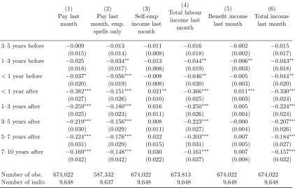
Our base model is Equation (1), which controls for individual fixed-effects. Results are reported in Table 4.26 Because we may observe zero pay, we estimate (1) in unlogged form and express the resulting coefficient estimates as a proportion of the mean pay of displaced workers atr = 0.
26In Appendix B we compare estimates from difference-in-differences, fixed-effects, fixed-effects with group trends and fixed-effects with individual trends.
Column (1) of Table4shows some evidence of a pre-displacement effect on pay which increases up to the point of displacement. This may either be due to pay falls within firms (for example, employers who are in difficulty paying lower wages) or due to selection of those who are going to be displaced into lower-paying firms. In the short-run, earnings fall by nearly 40% and then recover, but are still 17% lower than the counterfactual after 7–10 years.
If we compare column (1) and (2) we can gauge the extent to which these losses are caused by falls in monthly pay or differences in employment rates, because column (2) only considers those in employment. In the short-run after displacement, 60% of the earnings loss is due to lower employment rates, while 40% is due to lower pay (0.151/0.382). As time passes, a larger fraction of the earnings loss is accounted for by falls in monthly pay because a larger fraction of the displaced sample re-enters employment. In the final row we see that 88% (0.148/0.169) of the loss is accounted for by falls in monthly pay. These essentially replicate the patterns in the raw data shown in Figure3.
In column (3) we show that self-employment income is unimportant in mitigating either the short- or the long-run loss. There is a small increase in self-employment income of about 2% (albeit imprecisely estimated after one year). In column (4) we show that losses in total labour income (which includes self-employment income) are only slightly smaller than the losses in earnings shown in column (1).
In column (5) we report estimates of the impact of benefit income. Recall from panel (b) of Figure 2 that unemployment is typically a short-run experience, and as a result benefit effects are small and short-lived. Only 21% of the displaced sample report being unemployed one year after the displacement, and only 60% of these report receiving any benefit income. Those who are unemployed and in receipt of benefit receive an average of
reduced from 17% to 16%.
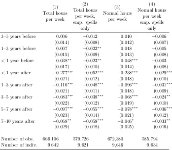
As we noted in the introduction, administrative data do not typically allow one to determine whether the fall in monthly pay is the result of falls in wages or falls in hours. In Table5we therefore report the corresponding estimates of the effect of displacement on normal and total hours. Normal hours are calculated from the question “Thinking about your (main) job, how many hours, excluding overtime and meal breaks, are you expected to work in a normal week?”. Total hours are the sum of normal hours and overtime hours, calculated from the question “How many hours overtime do you usually work in a normal week?”. Individuals who are not in employment are assigned zero hours of work.
Column (1) of Table 5should be compared with the same column (1) in Table4. In the year immediately following displacement monthly pay is 38% lower, while total hours are 28% lower. This is unsurprising since both include the large fraction of displaced workers who have zero hours of employment after displacement. After 10 years, monthly pay is 17% lower while total hours are 7% lower, suggesting that the majority of the fall in earnings is driven by lower wages rather than lower hours of work. Column (2) of Table5 shows how hours change conditional on being in employment. Here we see that hours of work in the jobs in which the displaced are re-employed are approximately 5% lower, and this fall is persistent over 10 years. This may partly be because displaced workers are more likely to be re-employed in part-time work (Farber, 1999). It may also be because these jobs offer less opportunity for overtime. In Column (4) we see that the fall in normal hours is about two percentage points smaller than the fall in total hours. Nevertheless, the results in Table5 show that, in the long-run (after 10 years), the majority of the fall in earnings is due to a fall in wages, not hours.
6.2 Matched samples
As shown in Table3, the treatment and control groups differ significantly in their observ-able characteristics before displacement occurs. To deal with this problem we use propen-sity score matching rather than regression to ensure that all members of the treatment and control group lie in the common region of the displacement propensity distribution. We match within cohort, so that an individual displaced in year c is matched only with
(1) Total hours
per week
(2) Total hours
per week, emp. spells
only
(3) Normal hours
per week
(4) Normal hours
per week emp. spells
only
3–5 years before 0.006 −0.012 0.010 −0.006
(0.014) (0.008) (0.012) (0.007)
1–3 years before 0.007 −0.022∗∗ 0.018 −0.005
(0.015) (0.009) (0.013) (0.008)
<1 year before 0.038∗∗ −0.023∗∗ 0.048∗∗∗ −0.003
(0.017) (0.010) (0.014) (0.008)
<1 year after −0.277∗∗∗ −0.052∗∗∗ −0.238∗∗∗ −0.029∗∗∗
(0.021) (0.012) (0.018) (0.010)
1–3 years after −0.116∗∗∗ −0.048∗∗∗ −0.096∗∗∗ −0.031∗∗∗
(0.021) (0.011) (0.018) (0.009)
3–5 years after −0.083∗∗∗ −0.038∗∗∗ −0.068∗∗∗ −0.024∗∗
(0.022) (0.012) (0.019) (0.010)
5–7 years after −0.097∗∗∗ −0.055∗∗∗ −0.078∗∗∗ −0.036∗∗∗
(0.023) (0.014) (0.021) (0.012)
7–10 years after −0.068∗∗ −0.058∗∗∗ −0.046∗ −0.033∗∗
(0.029) (0.018) (0.025) (0.016)
Number of obs. 666,106 579,726 672,380 585,794
[image:24.595.134.473.86.383.2]Number of indiv. 9,642 9,621 9,646 9,634
Table 5: FE estimates of the cost of displacement on individual hours. Table reports estimates of
δr from Equation (1) expressed as a proportion of the dependent variable of the treatment group
atr= 0. Both displaced and non-displaced groups are selected from those aged 16–60, who are in
employment in wavec.
individuals not displaced in yearc. In our base specification we impose the restriction that the treated and controls have common support, we allow for up to 10 nearest neighbours and we restrict the difference in the propensity to be no more than 0.005. In other words, the control group must have a propensity of being displaced less than 0.5% different from the treatment group. The propensity score is generated by a Probit model on a vectorxi
which contains measures of pre-displacement labour market history, firm tenure, firm size, sector of employment, occupation, union status, ethnic group, country of birth, region, sex, age, education and marital status. See TableC.1in AppendixC.
there-<12 months before displacement
5–6 years before displacement
Dc
i = 1 Dci= 0 p-value Dci= 1 Dci= 0 p-value
Employed 1.00 1.00 0.81 0.81 [0.800]
Self-employed 0.00 0.00 0.03 0.02 [0.365]
Unemployed 0.00 0.00 0.06 0.05 [0.076]
Other labour market state 0.00 0.00 0.10 0.12 [0.109]
Number of times interviewed before 6.06 6.00 [0.677] 3.71 3.66 [0.637] Number of times displaced before 0.23 0.23 [0.753] 0.13 0.16 [0.082] Displacement cohort (BHPS wave) 11.79 11.79 [1.000] 11.80 11.83 [0.827]
Tenure (years) 4.57 4.56 [0.988] 4.37 4.35 [0.949]
Firm employs<25 workers 0.38 0.38 [0.908] 0.29 0.35 [0.001] Works in manufacturing 0.33 0.33 [0.824] 0.35 0.34 [0.657] Works in manual occupation 0.45 0.45 [0.977] 0.46 0.48 [0.286]
Union member 0.35 0.35 [0.744] 0.40 0.39 [0.701]
Private sector 0.90 0.90 [0.949] 0.85 0.86 [0.545]
Works>30 hours per week 0.86 0.87 [0.386] 0.86 0.85 [0.832]
White ethnic group 0.92 0.92 [0.910] 0.96 0.96 [0.788]
Born in UK 0.95 0.95 [0.891] 0.95 0.95 [0.881]
Lives in South East 0.19 0.20 [0.666] 0.26 0.25 [0.690]
Female 0.40 0.40 [0.782] 0.43 0.41 [0.154]
Age (years) 38.95 38.99 [0.910] 35.91 35.40 [0.205]
Has degree 0.41 0.41 [0.818] 0.32 0.32 [0.779]
Married or cohabiting 0.69 0.70 [0.900] 0.66 0.66 [0.981]
Real monthly wage last month (£) 1525.66 1611.44 [0.016] 1225.67 1207.73 [0.663] Real self-employment income last month (£) 0.00 0.00 50.85 34.11 [0.482] Real monthly labour income last month (£) 1528.57 1582.94 [0.077] 1247.88 1239.28 [0.845] Real benefit income last month (£) 51.20 43.94 [0.098] 58.64 52.03 [0.188] Real monthly total income last month (£) 1626.55 1680.49 [0.092] 1351.91 1333.95 [0.682] Total hours per week (£) 39.67 40.05 [0.267] 32.83 33.45 [0.365] Normal hours per week (excl.overtime) 36.11 36.09 [0.942] 29.40 29.87 [0.435]
[image:25.595.94.510.86.497.2]N 1,413 11,125 894 7,074
Table 6: Characteristics of displaced and non-displaced workers before displacement, after
propen-sity score matching on characteristics atr= 0. “Real monthly pay” refers to pay from employment,
while “Real monthly earnings” also includes any self-employment earnings.
fore earnings atr = 0, but all other characteristics are insignificantly different between the displaced and non-displaced samples. The second column of Table 6 provides a stronger test of whether matching has successfully removed differences between the displaced and non-displaced groups, because we are comparing 5–6 years before the displacement oc-curs. Even here, matching has greatly reduced the differences between the displaced and non-displaced groups. There remains a very small difference in unemployment propensity (significant at 10%), but this difference is greatly reduced from the difference in unem-ployment propensity observed in the unmatched sample. There also remains a difference of 3 percentage points in the number of times displaced before, but in fact in this case it
(a) Employment
0.30 0.40 0.50 0.60 0.70 0.80 0.90 1.00
-10 -9 -8 -7 -6 -5 -4 -3 -2 -1 0 1 2 3 4 5 6 7 8 9 10 Time relative to displacement event (years)
(b) Unemployment
0.00 0.05 0.10 0.15 0.20 0.25 0.30 0.35 0.40
[image:26.595.115.492.84.240.2]-10 -9 -8 -7 -6 -5 -4 -3 -2 -1 0 1 2 3 4 5 6 7 8 9 10 Time relative to displacement event (years)
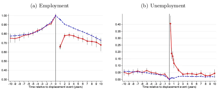
Figure 4: Probability of different self-reported labour market states before and after displacement 1991–2007, matched samples. 95% confidence intervals around the mean based on clustered standard errors.
is the non-displaced group who have a higher displacement rate from earlier periods.
A graphical illustration of the effectiveness of matching is provided by Figure 4, which can be compared with the unmatched comparison in panels (a) and (b) of Figure2. After matching, the non-displaced comparison group has almost identical pattern of pre-displacement employment and unemployment.
In Table 8 we report estimates of the effect of displacement on hours of work, after matching. As with the income results in Table7, matching reduces the estimated falls in hours. In particular, column (2) of Table 8 shows that those displaced workers who are re-employed have only marginally lower hours than the matched sample of non-displaced workers. In other words, the 10% fall in earnings shown in column (2) of Table7is entirely driven by falls in wages.
6.3 Selection into displacement
A potential bias to our estimates arises if there is a particular type of selection into displacement. If, for example, those who are displaced are selected on the basis of a negative shock to an unobservable characteristic (e.g. performance) which affect wages, then we will over-estimate the cost of displacement. As noted by Gibbons and Katz (1991), redundancies which are not caused by plant closure may allow for some discretion in terms of who gets displaced. However, we think that this bias is unlikely to be a major component of the observed estimate, for a number of reasons.
First, only a very specific type of selection into displacement threatens our identi-fication strategy. The selection has to be on the basis of a shock to performance which starts before r = 1, but it also has to be persistent from r = 1 onwards. If it reverts afterr = 1 then the long-term DiD estimates are unbiased. If selection into displacement is on the basis of permanent differences in performance then our DiD methodology deals with the selection. If the shock occurs beforer = 0 then we can test for it by examining the patterns of pre-displacement wages. In Table 7 estimates of δ prior to displacement are insignificantly different from zero until r = −1. If selection into displacement is on the basis of different pre-displacement trends in performance then our estimates which allow for differing trends deal with selection. In Table B.1 (column 3), we show that the difference in the pre-displacement trends are estimated to be close to zero.
Second, this particular type of selection seems much less likely to occur in a carefully matched sample. We have already seen from the matched samples that the time-series pattern of employment is remarkably similar for the displaced and non-displaced workers (see Figure4). This means that if there is still an unobserved difference in performance
(1) Pay last month (2) Pay last month, emp. spells only (3) Self-emp income last month (4) Total labour income last month (5) Benefit income last month (6) Total income last month
3–5 years before 0.016 0.009 −0.015∗ 0.008 0.000 0.009 (0.019) (0.019) (0.008) (0.021) (0.003) (0.021) 1–3 years before −0.002 0.000 −0.016∗ −0.018 −0.001 −0.019
(0.021) (0.020) (0.008) (0.022) (0.003) (0.022) <1 year before −0.040∗ −0.046∗∗ −0.010 −0.033 0.003 −0.031
(0.022) (0.022) (0.008) (0.022) (0.003) (0.022) <1 year after −0.367∗∗∗ −0.106∗∗∗ 0.015 −0.346∗∗∗ 0.017∗∗∗ −0.310∗∗∗
(0.028) (0.029) (0.011) (0.028) (0.004) (0.027) 1–3 years after −0.230∗∗∗ −0.145∗∗∗ 0.010 −0.217∗∗∗ 0.011∗∗∗ −0.191∗∗∗
(0.027) (0.027) (0.011) (0.028) (0.004) (0.027) 3–5 years after −0.179∗∗∗ −0.119∗∗∗ −0.000 −0.181∗∗∗ 0.004 −0.165∗∗∗
(0.032) (0.034) (0.011) (0.031) (0.005) (0.030) 5–7 years after −0.172∗∗∗ −0.112∗∗∗ 0.005 −0.156∗∗∗ 0.010∗ −0.132∗∗∗
(0.036) (0.038) (0.015) (0.037) (0.006) (0.035) 7–10 years after −0.120∗∗ −0.101∗ 0.014 −0.116∗∗ 0.007 −0.105∗∗
(0.051) (0.058) (0.024) (0.049) (0.009) (0.046)
[image:28.595.92.514.98.369.2]Number of obs. 155,280 133,138 155,280 155,238 155,280 155,280 Number of indiv. 6,035 6,035 6,035 6,035 6,035 6,035
Table 7: PSM estimates of the cost of displacement on individual earnings and income.
(1) Total hours per week (2) Total hours per week, emp. spells only (3) Normal hours per week (4) Normal hours per week emp. spells only
3–5 years before −0.011 −0.013 −0.006 −0.007
(0.014) (0.010) (0.012) (0.008)
1–3 years before −0.023∗∗ −0.015∗ −0.010 −0.002
(0.011) (0.009) (0.009) (0.007)
<1 year before −0.009 −0.009 0.000 0.001
(0.008) (0.008) (0.007) (0.007)
<1 year after −0.315∗∗∗ −0.022∗∗ −0.277∗∗∗ −0.013
(0.015) (0.010) (0.013) (0.009)
1–3 years after −0.134∗∗∗ −0.020∗∗ −0.120∗∗∗ −0.017∗∗
(0.014) (0.010) (0.012) (0.008)
3–5 years after −0.092∗∗∗ −0.007 −0.089∗∗∗ −0.014
(0.017) (0.012) (0.015) (0.010)
5–7 years after −0.101∗∗∗ −0.020 −0.096∗∗∗ −0.024∗
(0.021) (0.015) (0.018) (0.012)
7–10 years after −0.056∗ −0.012 −0.050∗ −0.011
(0.029) (0.024) (0.026) (0.019)
Number of obs. 153,410 131,353 154,912 132,798
Number of indiv. 6,033 6,032 6,035 6,035
[image:28.595.132.469.424.723.2]shocks between r = 0 and r = 1 it would have to be entirely uncorrelated with earlier shocks.
Third, redundancy criteria in the UK are made on the basis of organisational re-quirements (such as which jobs must be lost) rather than the performance of individual workers. In the UK, poorly-performing workers can normally be dismissed only after formal dismissal procedures.
Finally, if negative selection were a major problem which affected self-reported mea-sures of displacement, we expect that estimates from survey data will be systematically larger than estimates from administrative data which use externally verified measures of displacement. The evidence from Couch and Placzek’s (2010) literature review does not support this assertion.
To further examine the issue of selection in the data, we consider the distinction between those those whose job spell ended due to redundancy and those that ended due to dismissal. We would expect that selection into displacement as a result of a shock to performance will be more likely for those who are dismissed. Of the 2,499 displacements, the vast majority (2,225) are “made redundant” and only 264 are “dismissed/sacked”. We perform propensity score matching separately on each sub-group and estimate a difference-in-difference model on the matched samples.
Table 9 reports the results. Columns (1) and (2) repeat the base model for all displacements. Columns (5) and (6) report the estimates for the “dismissal” sample. These estimates are substantially larger, particularly for periods further away from the displacement date. Dismissed workers’ wage losses are estimated to be around 30% of the pre-displacement wage after 10 years, compared to only 10% for workers made redundant, shown in columns (3) and (4). These results are consistent with the hypothesis that selection into dismissal is more likely than selection into redundancy. However, the very small number of dismissals means that the results would not change greatly if they are excluded.
All displacements Made redundant Dismissed/sacked (1)
Pay last month
(2) Pay last month, emp.
spells only
(3) Pay last
month
(4) Pay last month, emp.
spells only
(5) Pay last
month
(6) Pay last month, emp.
spells only
3–5 years before 0.016 0.009 0.034∗ 0.021 −0.061 −0.042 (0.019) (0.019) (0.019) (0.020) (0.078) (0.079) 1–3 years before −0.002 0.000 0.024 0.018 −0.094 −0.038
(0.021) (0.020) (0.022) (0.022) (0.080) (0.080) <1 year before −0.040∗ −0.046∗∗ −0.009 −0.013 −0.109 −0.091
(0.022) (0.022) (0.023) (0.024) (0.081) (0.088) <1 year after −0.367∗∗∗ −0.106∗∗∗ −0.351∗∗∗ −0.094∗∗∗ −0.421∗∗∗ −0.086
(0.028) (0.029) (0.030) (0.031) (0.090) (0.110) 1–3 years after −0.230∗∗∗ −0.145∗∗∗ −0.207∗∗∗ −0.125∗∗∗ −0.335∗∗∗ −0.194∗∗
(0.027) (0.027) (0.029) (0.029) (0.093) (0.095) 3–5 years after −0.179∗∗∗ −0.119∗∗∗ −0.153∗∗∗ −0.098∗∗ −0.427∗∗∗ −0.338∗∗∗
(0.032) (0.034) (0.036) (0.038) (0.115) (0.121) 5–7 years after −0.172∗∗∗ −0.112∗∗∗ −0.158∗∗∗ −0.118∗∗∗ −0.404∗∗∗ −0.358∗∗∗
(0.036) (0.038) (0.039) (0.042) (0.142) (0.135) 7–10 years after −0.120∗∗ −0.101∗ −0.098∗ −0.093 −0.300∗ −0.296∗ (0.051) (0.058) (0.054) (0.063) (0.176) (0.162)
[image:30.595.91.513.82.355.2]Number of obs. 155,280 133,138 142,953 122,975 13,476 10,912 Number of indiv. 6,035 6,035 5,651 5,651 1,087 1,087
Table 9: DiD estimates on matched samples, comparison of displacement type.
6.4 Losses by cohort
The pooled models impose the restriction that the effect of displacement relative to the displacement date is the same for all cohorts. For example, the effect of displacement in 2000 on an individual’s earnings in 2002 is the same as the effect of displacement in 2002 on an individual’s earnings in 2004. The structure of our data implies that estimates of the loss for periods further from the displacement event are identified by earlier cohorts, since later cohorts are followed for a shorter period of time. Davis and von Wachter (2011) show that the cost of displacement varies substantially across cohorts, depending in particular on economic conditions at the time of displacement: workers displaced in a downturn suffer much larger losses. Thus, it is possible that the slow recovery in earnings may be driven by that fact that earlier cohorts were displaced during the weaker labour market in the early 1990s. In Figure5 we report estimates of (1) for four displacement cohorts. To maintain reasonable sample size, each cohort comprises three years: 1996–1998, 1999– 2001, 2002–2005 and 2006–2008.
(a) Pay last month
96-98
99-01
02-04 05-07
-700 -600 -500 -400 -300 -200 -100 0 100
FE estimate of earnings change (£)
-5 -4 -3 -2 -1 0 1 2 3 4 5 6 7 8 9 10 11 Years relative to displacement year
(b) Pay last month (employment spells only)
96-98 99-01 02-04 05-07
-700 -600 -500 -400 -300 -200 -100 0 100
FE estimate of earnings change (£)
[image:31.595.109.485.87.239.2]-5 -4 -3 -2 -1 0 1 2 3 4 5 6 7 8 9 10 11 Years relative to displacement year
Figure 5: FE estimates by cohort (each cohort contains three years). Dotted line indicates average across all cohorts.
result of the fact that business cycle fluctuations were small over the sample period (which pre-dates the “Great Recession” of 2008–2009), and therefore the time-series pattern of earnings recovery is unlikely to be affected by the business cycle.
6.5 Further robustness checks
Our strategy in this paper is to provide estimates of the cost of displacement based on the largest sample of displaced workers. In part this is driven by the relatively small numbers of displaced workers observed in the survey data, but also by a desire to provide estimates which are representative of all displacements. In contrast, much of the literature, following JLS, restricts the group of displaced workers in various dimensions, such as age, firm tenure and the observation of post-displacement earnings. In Appendix D we investigate the impact of various sampling decisions on the estimated loss. We show that most of these decisions have only a small impact on estimated losses, consistent with findings from the US, as in von Wachter et al. (2009). The most significant sampling decision is that which relates to the control group. If the control group is restricted to include only those who remain with their employer fromr > 0 onwards, estimated losses are larger and there is no recovery in relative pay because the control group have faster growth in pay.