Rotational superradiant scattering in a vortex flow

Rotational superradiant scattering in a vortex flow

Theo Torres1_{, Sam Patrick}1_{, Antonin Coutant}1_{, Maur´ıcio Richartz}2_{, Edmund W. Tedford}3 _{& Silke} Weinfurtner1,4,5

1_{School of Mathematical Sciences, University of Nottingham, University Park, Nottingham, NG7}

2RD, UK

2_{CMCC - Centro de Matem´atica, Computac¸˜ao e Cognic¸˜ao, Universidade Federal do ABC}

(UFABC), 09210-170 Santo Andr´e, S˜ao Paulo, Brazil

3_{Department of Civil Engineering, University of British Columbia, 6250 Applied Science Lane,}

Vancouver, Canada V6T 1Z4

4_{School of Physics and Astronomy, University of Nottingham, Nottingham, NG7 2RD, UK.}

5_{Centre for the Mathematics and Theoretical Physics of Quantum Non-Equilibrium Systems,}

Uni-versity of Nottingham, Nottingham, NG7 2RD, UK.

on a draining fluid constitute an analogue of a black hole5–10_{, but also on hydrodynamics, 9} due to its close relation to over-reflection instabilities11–13_{. 10}

In water, perturbations of the free surface manifest themselves by a small change ξ(t,x) 11 of the water height. On a flat bottom, and in the absence of flow, linear perturbations are well 12 described by superpositions of plane waves of definite frequencyf(Hz) and wave-vectork(rad/m). 13 When surface waves propagate on a changing flow, the surface elevation is generally described by 14 the sum of two contributionsξ=ξI+ξS, whereξIis theincidentwave produced by a source, e.g. a 15 wave generator, whileξS is thescattered wave, generated by the interaction between the incident 16 wave and the background flow. In this work, we are interested on the properties of this scattering 17 on a draining vortex flow which is assumed to beaxisymmetricandstationary. At the free surface, 18 the velocity field is given in cylindrical coordinates byv=vrer+vθeθ+vzez. 19

Due to the symmetry, it is appropriate to describe ξI andξS using polar coordinates(r, θ). 20 Any waveξ(t, r, θ)can be decomposed into partial waves10, 14, 21

ξ(t, r, θ) = Re "

X

m∈Z

Z ∞

0

ϕf,m(r)

e−2iπf t+imθ √

r df

#

, (1)

oscillatory solutions, 27

ϕ(r) = Aine−ikr+Aouteikr, (2)

wherek = _||k_||2 is the wave-vector norm. This describes the superposition of an inward wave of 28 (complex) amplitude Ain propagating towards the vortex, and an outward one propagating away 29 from it with amplitude Aout. These coefficients are not independent. The Ain’s, one for eachf 30 and m component, are fixed by the incident part ξI. If the incident wave is a plane wave ξ = 31

ξ0e−2iπf t+ik·x, then the partial amplitudes are given byAin = ξ0eimπ+iπ/4/

√

2πk. In other words, 32 a plane wave is a superposition containingallazimuthal waves, something that we have exploited 33 in our experiment. On the contrary,Aout depends on the scattered partξS, and how precisely the 34 waves propagate in the centre and interact with the background vortex flow. In the limit of small 35 amplitudes, there is a linear relation between the Ain’s and Aout’s, and by the symmetries of the 36

flow, differentf andmdecouple10, 15. 37

This allows us to define the reflection coefficient at fixedf and m as the ratio between the 38

outward(Jout)and inward(Jin)energy fluxes, 39

R=

r Jout

Jin

. (3)

In the linear approximation, the wave energy is a quadratic quantity in wave amplitude, andR is 40

proportional to the amplitude ratio|Aout/Ain|. 41

the vortex during the process. 45

We conducted our experiment in a 3 mlong and1.5 mwide rectangular water tank. Water 46 is pumped continuously in from one end corner, and is drained through a hole (4 cmin diameter) 47 in the middle. The water flows in a closed circuit. We first establish a stationary rotating draining 48 flow by setting the flow rate of the pump to37.5 ± 0.5`/minand waiting until the depth (away 49 from the vortex) is steady at6.25 _± 0.05 cm. We then generate plane waves from one side of 50 the tank, with an excitation frequency varying from2.87 Hzto 4.11 Hz. On the side of the tank 51 opposite the wave generator, we have placed an absorption beach (we have verified that the amount 52 of reflection from the beach is below 5% in all experiments). We record the free surface with a 53 high speed 3D air-fluid interface sensor. The sensor is a joint-invention16_{(patent No. DE 10 2015}

54

001 365 A1) between The University of Nottingham and EnShape GmbH (Jena, Germany). 55

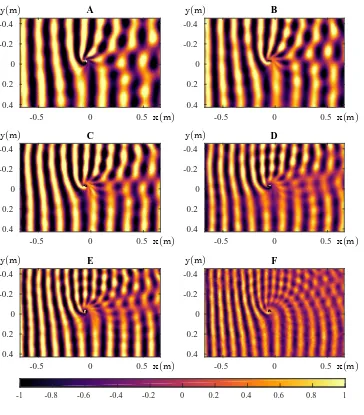
bathtub flow models10, 17_{. We also observe that incident waves have more wave fronts on the upper}

65

half of the vortex in comparison with the lower half - see the various wave characteristics in panels 66 (A-F) inFig. 1. This angular phase shift is analogous to the Aharonov-Bohm effect, and has been 67 observed in previous water wave experiments18, 19_{. Our detection method allows for a very clear}

68

visualization of this effect. 69

The second filter is the polar Fourier transform, which selects a specific azimuthal wave num- 70 berm, and allows the radial profileϕ(r)to be determined. To extract the reflection coefficient, we 71 use a windowed Fourier transform of the radial profileϕ(r). The windowing is done on the inter- 72 val[rmin, rmax]. When rminis large enough, the radial profile ϕcontains two Fourier components 73 [see Eq. (2)], one of negative k (inward wave), and one of positive k (outward wave). The ratio 74 between their two amplitudes gives us the reflection coefficient (up to the energy correction, see 75 Methods - Wave energy). In order to better resolve the two peaks, we have applied a Hamming 76 window on the radial profile over the interval[rmin, rmax]. In all experiments,rmin '0.15 m, while 77

rmax ' 0.39 m. We also point out that the minimum radius such that the radial profile reduces to 78 Eq. (2) increases withm. With the size of our window, and the wavelength range of the experiment, 79

we can resolve with confidencem =₋2,₋1,0,1,2. 80

positive m’s have a reflection coefficient close to 1. In some cases this reflection is above one, 85 meaning that the corresponding mode has been amplified while scattering on the vortex. To confirm 86 this amplification we have repeated the same experiment 15 times at the frequencyf = 3.8 Hzand 87 water heighth0 = 6.25 ± 0.05 cm, for which the amplification was the highest. We present the 88 result onFig. 3. On this figure we clearly observe that the modesm= 1andm = 2are amplified 89 by factorsRm=1 ∼1.09±0.03, andRm=2 ∼1.14±0.08respectively. OnFigs. 2and3, we have 90 also shown the reflection coefficients obtained for a plane wave propagating on standing water 91 of the same depth. Unlike what happens in the presence of a vortex, the reflection coefficients 92 are all below 1 (within error bars). For low frequencies it is close to 1, meaning that the wave is 93 propagating without losses, while for higher frequencies it decreases due to a loss of energy during 94

the propagation, i.e. damping. 95

The origin of this amplification can be explained by the presence of negative energy waves 96

20, 21_{. Negative energy waves are excitations that lower the energy of the whole system (i.e.}

back-97

ground flow and excitation) instead of increasing it. In our case, the sign of the energy of a wave is 98 given by the angular frequency in the fluid frameωfluid. If the fluid rotates with an angular velocity 99

Ω(r), in rad/s, we have ωfluid = 2πf −mΩ(r). At fixed frequency, when the fluid rotates fast 100 enough, the energy becomes negative. If part of the wave is absorbed in the hole, carrying negative 101 energy, the reflected part must come out with a higher positive energy to ensure conservation of the 102 total energy2_{. Using Particle Imaging Velocimetry (PIV), we have measured the velocity field of}

103

range. 106

Our experiment demonstrates that a wave scattering on a rotating vortex flow can carry away 107 more energy than the incident wave brings in. Our results show that the phenomenon of superradi- 108 ance is very robust and requires few ingredients to occur, namely high angular velocities, allowing 109 for negative energy waves, and a mechanism to absorb these negative energies. For about half of 110 the frequency range, our results confirm superradiant amplification despite a significant damping 111 of the waves. The present experiment does not reveal the mechanism behind the absorption of the 112 negative energies. The likely possibilities are that they are dissipated away in the vortex throat, 113 in analogy to superradiant cylinders4, 22_{, that they are trapped in the hole}23_{and unable to escape,}

114

similarly to what happens in black holes 24, 25_{, or a combination of both. A possible way to}

dis-115

tinguish between the two in future experiments would be to measure the amount of energy going 116

x(m)

y(m) E

-0.5 0 0.5

-0.4 -0.2 0 0.2 0.4 x(m) y(m) A

-0.5 0 0.5

-0.4 -0.2 0 0.2 0.4 x(m) y(m) B

-0.5 0 0.5

-0.4 -0.2 0 0.2 0.4 x(m) y(m) C

-0.5 0 0.5

-0.4 -0.2 0 0.2 0.4 x(m) y(m) D

-0.5 0 0.5

-0.4 -0.2 0 0.2 0.4 x(m) y(m) F

-0.5 0 0.5

-0.4

-0.2

0

0.2

0.4

-1 -0.8 -0.6 -0.4 -0.2 0 0.2 0.4 0.6 0.8 1

118

Figure 1|Wave characteristics of the surface perturbationξ, filtered at a single frequency, for six 119 different frequencies. The frequencies are2.87 Hz (A), 3.04 Hz (B), 3.27 Hz (C), 3.45 Hz (D), 120

3.70 Hz(E), and4.11 Hz(F). The horizontal and vertical axis are in metres (m), while the color 121 scale is in millimetres (mm). The patterns show the interfering sum of the incident wave with the 122 scattered one. The waves are generated on the left side and propagate to the right across the vortex 123

f (Hz)

2.6 2.8 3 3.2 3.4 3.6 3.8 4 4.2

R

0 0.5

1 1.5

without vortex with vortex, m= +2 with vortex, m= +1 with vortex, m= 0 with vortex, m= -1 with vortex, m= -2

125

Figure 2|Reflection coefficients for various frequencies and variousm’s. For the vortex experi- 126 ments the statistical average is taken over 6 repetitions, except forf = 3.70 Hzwhere we have 15 127 repetitions. The purple line (star points) shows the reflection coefficients of a plane wave in stand- 128 ing water of the same height. We observe a significant damping for the frequencies above 3Hz (see 129 Fig. 2). In future experiments, we hope to reduce this damping by working with purer water 26_.

130

instead of6, and overm=₋2. . .2(the reflection coefficient of a plane wave on standing water is 132 in theory independent ofm, see alsoFig. 3). The errors bars indicate the standard deviation over 133 these experiments, the energy uncertainty and the standard deviation over several centre choices 134 (see Methods). The main contribution comes from the variability of the value of the reflection 135 coefficient for different repetitions of the experiment. We have also extracted the signal-to-noise 136 ratio for each experiment, and its contribution to the error bars is negligible (see Method - Data 137

m

-2 -1 0 1 2

R

0 0.2 0.4 0.6 0.8 1 1.2 1.4

with vortex without vortex

139

Figure 3 | Reflection coefficients for different m’s, for the frequency f = 3.70 Hz(stars). We 140 have also shown the reflection coefficients for plane waves without a flow, at the same frequency 141 and water height (diamonds). We see that the plane wave reflection coefficients are identical for all 142

m’s, and all below 1 (within error bars). The statistic has been realized over 15 experiments. Error 143

0 0.02 0.04 0.06

r

(m)

v

(m

/

s)

C

0 0.02 0.04 0.06

r

(m)

~

v

(m

/

s)

D

0 0.02 0.04 0.06

r

(m)

+

(r

a

d

/

s)

A

B

-5 0 5

x

(cm)

y

(c

m

)

151 1. Brito, R., Cardoso, V. & Pani, P. Superradiance. Lect. Notes Phys.906, 1–237 (2015). 152

2. Richartz, M., Weinfurtner, S., Penner, A. J. & Unruh, W. G. Generalized superradiant scatter- 153

ing. Phys. Rev. D80, 124016 (2009). 154

3. Zel’Dovich, Y. B. Generation of Waves by a Rotating Body. JETP Lett.14, 180–181 (1971). 155

4. Zel’Dovich, Y. B. Amplification of Cylindrical Electromagnetic Waves Reflected from a Ro- 156

tating Body. Sov. Phys. JETP35, 1085–1087 (1972). 157

5. Unruh, W. Experimental black hole evaporation. Phys. Rev. Lett.46, 1351–1353 (1981). 158

6. Visser, M. Acoustic black holes: horizons, ergospheres and Hawking radiation. Classical and 159

Quantum Gravity15, 1767–1791 (1998). 160

7. Sch¨utzhold, R. & Unruh, W. G. Gravity wave analogues of black holes. Phys. Rev. D 66, 161

044019 (2002). 162

8. Weinfurtner, S., Tedford, E. W., Penrice, M. C. J., Unruh, W. G. & Lawrence, G. A. Measure- 163 ment of stimulated hawking emission in an analogue system. Phys. Rev. Lett. 106, 021302 164

(2011). 165

9. Steinhauer, J. Observation of thermal Hawking radiation and its entanglement in an analogue 166

black hole. Nature Phys.12, 959–965 (2016). 167

10. Dolan, S. R. & Oliveira, E. S. Scattering by a draining bathtub vortex.Phys. Rev.D87, 124038 168

11. Acheson, D. J. On over-reflexion. Journal of Fluid Mechanics77, 433–472 (1976). 170

12. Kelley, D. H., Triana, S. A., Zimmerman, D. S., Tilgner, A. & Lathrop, D. P. Inertial waves 171 driven by differential rotation in a planetary geometry. Geophysical and Astrophysical Fluid 172

Dynamics101, 469–487 (2007). 173

13. Fridman, A.et al. Over-reflection of waves and over-reflection instability of flows revealed in 174 experiments with rotating shallow water. Physics Letters A372, 4822–4826 (2008). 175

14. Newton, R. G. Scattering theory of waves and particles(Courier Dover Publications, 1982). 176

15. Richartz, M., Prain, A., Liberati, S. & Weinfurtner, S. Rotating black holes in a draining 177 bathtub: superradiant scattering of gravity waves. Phys. Rev. D91, 124018 (2015). 178

16. Schaffer, M., Große, M. & Weinfurtner, S. Verfahren zur 3d-vermessung von fl¨ussigkeiten und 179 gelen (2016). URL http://google.com/patents/DE102015001365A1?cl=zh. 180

DE Patent App. DE201,510,001,365. 181

17. Dolan, S. R., Oliveira, E. S. & Crispino, L. C. B. Aharonov-Bohm effect in a draining bathtub 182

vortex. Physics Letters B701, 485–489 (2011). 183

18. Berry, M., Chambers, R., Large, M., Upstill, C. & Walmsley, J. Wavefront dislocations in the 184 aharonov-bohm effect and its water wave analogue. European Journal of Physics1, 154–162 185

(1980). 186

20. Stepanyants, Y. A. & Fabrikant, A. Propagation of waves in shear flows. Physical and Math- 189

ematical Literature Publishing Company, Russian Academy of Sciences, Moscow(1996). 190

21. Coutant, A. & Parentani, R. Undulations from amplified low frequency surface waves. Phys. 191

Fluids26, 044106 (2014). 192

22. Cardoso, V., Coutant, A., Richartz, M. & Weinfurtner, S. Detecting rotational superradiance 193

in fluid laboratories. Phys. Rev. Lett.117, 271101 (2016). 194

23. Basak, S. & Majumdar, P. ‘Superresonance’ from a rotating acoustic black hole. Class. Quant. 195

Grav.20, 3907–3914 (2003). 196

24. Misner, C. Stability of Kerr black holes against scalar perturbations. Bulletin of the American 197

Physical Society17, 472 (1972). 198

25. Starobinsky, A. A. Amplification of waves during reflection from a rotating black hole. Sov. 199

Phys. JETP37, 28–32 (1973). 200

26. Przadka, A., Cabane, B., Pagneux, V., Maurel, A. & Petitjeans, P. Fourier transform profilom- 201 etry for water waves: how to achieve clean water attenuation with diffusive reflection at the 202

water surface? Experiments in fluids52, 519–527 (2012). 203

27. B¨uhler, O. Waves and mean flows(Cambridge University Press, 2014). 204

28. Richartz, M., Prain, A., Weinfurtner, S. & Liberati, S. Superradiant scattering of dispersive 205

29. Coutant, A. & Weinfurtner, S. The imprint of the analogue Hawking effect in subcritical flows. 207

Phys. Rev. D94, 064026 (2016). 208

Methods 209

Wave energy. To verify that the observed amplification increases the energy of the wave, we 210 compare the energy current of the inward wave with respect to the outward one. Since energy is 211 transported by the group velocity vg, the energy current is given by J = g ωfluid−1 vg|A|2/f (up to 212 the factor 1/f, this is the wave action, an adiabatic invariant of waves 27–29). If the background 213 flow velocity is zero, then the ratioJout/Jinis simply|Aout/Ain|2. However, in the presence of the 214 vortex, we observe from our radial profiles ϕ(r) [defined in equation (1)] that the wave number 215 of the inward and outward waves are not exactly opposite. The origin of this (small) difference is 216 that the flow velocity is not completely negligible in the observation window. It generates a small 217 Doppler shift that differs depending on whether the wave propagates against or with the flow. In 218 this case, the ratio of the energy currents picks up a small correction with respect to the ratio of the 219

amplitudes, namely, 220

Jout Jin = ωin fluidvoutg

ωout fluidving

Aout Ain 2 . (4)

To estimate this factor, we assume that the flow varies slowly in the observation window, such 221 that ωfluid obeys the usual dispersion relation of water waves, ω2fluid = gktanh(h0k). (This 222 amounts to a WKB approximation, and capillarity is neglected.) Under this assumption, the 223 group velocity is the sum of the group velocity in the fluid frame, given by the dispersion rela- 224 tion, vfluid

g = ∂k

p

needed for the energy ratio (4) splits into two:vg =vgfluid+vr. The first term is obtained only with 226 the values ofkinandkout, extracted from the radial Fourier profiles. The second term requires the 227 value ofvr, which we do not have to a sufficient accuracy. However, using the PIV data, we see 228 that the contribution of this last term amounts to less than1%in all experiments (this uncertainty 229

is added to the error bars onFigs. 2and3). 230

Data analysis. We record the free surface of the water in a region of1.33 m_×0.98 mover the 231 vortex during 13.2 s. From the sensor we obtain 248 reconstructions of the free surface. These 232 reconstructions are triplets Xij, Yij and Zij giving the coordinates of 640 × 480 points on the 233 free surface. Because of the shape of the vortex, and noise, parts of the free surface cannot be 234 seen by our sensor, resulting in black spots on the image. Isolated black spots are corrected by 235 interpolating the value of the height using their neighbours. This procedure is not possible in the 236

core of the vortex and we set these values to zero. 237

To filter the signal in frequency, we first crop the signal in time so as to keep an integer 238 number of cycles to reduce spectral leakage. We then select a single frequency corresponding to 239 the excitation frequency f0. After this filter, we are left with a 2-dimensional array of complex 240 values, encoding the fluctuations of the water heightξ(Xij, Yij)at the frequencyf0. ξ(Xij, Yij)is 241 defined on the gridsXij, andYij, whose points are not perfectly equidistant (this is due to the fact 242 that the discretization is done by the sensor software in a coordinate system that is not perfectly 243

parallel to the free surface). 244

nates. For this we need to find the centre of symmetry of the background flow. We define our 246 centre to be the centre of the shadow of the vortex, averaged over time (the fluctuations in time are 247 smaller than a pixel). To verify that this choice does not affect the end result, we performed a sta- 248 tistical analysis on different centre choices around this value, and added the standard deviation to 249 the error bars. Once the centre is chosen, we perform a discrete Fourier transform on the irregular 250 grid(Xij, Yij). We create an irregular polar grid(rij, θij)and we compute 251

ϕm(rij) =

√_r

ij

2π X

j

ξ(rij, θij)e−imθij∆θij, (5)

where∆θij = (∆Xij∆Yij)/(rij∆rij)is the line element along a circle of radiusrij. 252

To extract the inward and outward amplitudesAin andAout, we compute the radial Fourier 253 transformϕ˜m(k) =

R

ϕm(r)e−ikrdr over the window[rmin, rmax]. Due to the size of the window 254 compared to the wavelength of the waves, we can only capture a few oscillations in the radial 255 direction, typically between 1 and 3. This results in broad peaks around the values kin and kout 256 of the inward and outward components. We assume that these peaks contain only one wavelength 257 (no superposition of nearby wavelengths), which is corroborated by the fact that we have filtered 258 in time, and the dispersion relation imposes a single wavelength at a given frequency. To reduce 259 spectral leakage, we use a Hamming window function on[rmin, rmax], defined as 260

W(n) = 0.54−0.46 cos2πn N

, (6)

wherenis the pixel index running from1toN. This window is optimized to reduce the secondary 261 lobe, and allows us to better distinguish peaks with different amplitudes 31_{. InSupplementary}

262

and the raw radial profiles and how they are approximated by Eq. (2) (right column). 264

We also extracted the signal-to-noise ratio by comparing the standard deviation of the noise 265 to the value of our signal. It is sufficiently high to exclude the possibility that the amplification we 266 observed is due to a noise fluctuation, and its contribution is negligible compared to other sources 267

of error. 268

PIV measurements. Close to the vortex core, the draining bathtub vortex is cylindrically sym- 269 metric to a good approximation. An appropriate choice of coordinates is, therefore, cylindrical 270 coordinates(r, θ, z). The velocity field will be independent of the angleθ and can be expressed as 271

v(r, z) = vr(r, z)er+vθ(r, z)eθ+vz(r, z)ez. (7)

We are specifically interested in the velocity field at the free surface z = h(r). When the free 272 surface is flat, h is constant and the vertical velocity vz vanishes. When the surface is not flat, 273 the vz component can be deduced from vr using the free surface profile h(r) and the equation 274

vz(r, h(r)) = (∂rh)vr|z=h. To obtain an estimate ofvz, we use a simple model for the free surface 275 shape32_,

276

h(r) =h0

1− r

2 a

r2

, (8)

where h0 is the water height far from the vortex and ra is the radial position at which the free 277 surface passes through the sink hole. This approximation captures the essential features of our 278 experimental data. The components vr and vθ are determined through the technique of Particle 279 Imaging Velocimetry (PIV), implemented through the Matlab extension PIVlab33, 34. The tech- 280

The flow is seeded with flat paper particles of mean diameter d = 2 mm. The particles 282 are buoyant which allows us to evaluate the velocity field exclusively at the free surface. The 283 amount by which a particle deviates from the streamlines of the flow is given by the velocity lag 284

Us =d2(ρ−ρ0)a/18µ(ref.33), whereρis the density of a particle,ρ0 is the density of water,µis 285 the dynamic viscosity of water andais the acceleration of a particle. For fluid accelerations in our 286 system this is at most of the order10−4_{m/s, an order of magnitude below the smallest velocity in}

287

the flow. Thus we can safely neglect the effects of the velocity lag when considering the motions 288

of the particles in the flow. 289

The surface is illuminated using two light panels positioned at opposite sides of the tank. 290 The flow is imaged from above using a Phantom Miro Lab 340 high speed camera at a frame rate 291 of800 fpsfor an exposure time of1200µs. The raw images are analysed usingPIVlabby taking a 292 small window in one image and looking for a window within the next image which maximizes the 293 correlation between the two. By knowing the distance between these two windows and the time 294 step between two images, it is possible to give each point on the image a velocity vector. This 295 process is repeated for all subsequent images and the results are then averaged in time to give a 296

mean velocity field. 297

the order of|˜vl_/v

g|, where˜vlis the angular Fourier component of azimuthal numberl=m−m0. 303 This ratio is smaller than 3% in all experiments. To obtain the radial profiles of vr and vθ, we 304 integrate them over the angleθ. InFigs. 4Cand4Dwe showvθand the inward velocity tangent to 305 the free surface,v˜r =−

p v2

r+vz2, as functions ofr. 306

We compare the data forvθwith the Lamb vortex32, 307

vθ(r, h) =

Ω0r20

r

1₋exp

−r

2

r2 0

, (9)

whereΩ0 is the maximum angular velocity in the rotational core of characteristic radiusr0. (For 308

vθ we have Ω0 = 69.4 rad/s and r0 = 1.34 cm, and for vr we have Ω0 = −4.52 rad/s and 309

r0 = 1.39 cm.) Outside the vortex core, this model reduces to the characteristic1/rdependence 310 of an incompressible, irrotational flow depending only on r. By observing that vθ and vr exhibit 311 similar qualitative behaviour, vr is also fitted with a model of the form of equation (9). Figs. 4C 312 and4Dshow that equation (9) captures the essential features of the measured velocity profiles. The 313 angular velocity of the flow is given byΩ(r) = vθ/rwhich is shown inFig. 4A. From this plot it 314 is clear thatΩreaches large enough values to be consistent with the detection of superradiance. 315

The data that support the plots within this paper and other findings of this study are available 316

from the corresponding author upon reasonable request. 317

31. Prabhu, K. Window functions and their applications in signal processing(CRC Press, 2013).

32. Lautrup, B.Physics of continuous matter: exotic and everyday phenomena in the macroscopic

33. Thielicke, W. The flapping flight of birds. Ph.D. thesis, University of Groningen (2014).

34. Thielicke, W. & Stamhuis, E. PIVlab–towards user-friendly, affordable and accurate digital particle image velocimetry in MATLAB. Journal of Open Research Software2, e30 (2014).

Acknowledgements We are indebted to the technical and administrative staff in the School of Physics &

Astronomy where our experimental setup is hosted. In particular, we want to thank Terry Wright and Tommy

Napier for their support, hard work and sharing their technical knowledge and expertise with us to set up

the experiment in Nottingham. Furthermore we would like to thank Bill Unruh, Stefano Liberati, Joseph

Niemela, Luis Lehner, Vitor Cardoso, Michael Berry, Vincent Pagneux, Daniele Faccio, Fedja Orucevic,

J¨org Schmiedmayer and Thomas Fernholz for discussions regarding the experiment, and we wish to thank

Michael Berry, Vitor Cardoso, Daniele Faccio, Luis Lehner, Stefano Liberati, and Bill Unruh for comments

on the paper. Although all experiments have been conducted at The University of Nottingham, the initial

stages of the experiment took place at ICTP / SISSA in Trieste (Italy) and would not have been possible

without the support by Joseph Niemela, Stefano Liberati and Guido Martinelli. S. W. would like to thank

Matt Penrice, Angus Prain, Miltcho Danailov, Ivan Cudin, Henry Tanner, Zack Fifer, Andreas Finke, and

Dylan Russon for their contributions at different stages of the experiment. S. W. would also like to thank

Thomas Sotiriou for the many discussions on all aspects of the project.

A. C. acknowledges funding received from the European Union’s Horizon 2020 research and innovation

programme under the Marie Sklodowska Curie grant agreement No 655524. M. R. acknowledges financial

support from the S˜ao Paulo Research Foundation (FAPESP), Grants No. 2005/04219-0, No.

2010/20123-1, No. 2013/09357-9, No. 2013/15748-0 and No. 2015/14077-0. M. R. and Ted T. are also grateful to

ac-knowledges financial support provided under the Royal Society University Research Fellow (UF120112),

the Nottingham Advanced Research Fellow (A2RHS2), the Royal Society Project (RG130377) grants and

the EPSRC Project Grant (EP/P00637X/1). The initial stages of the experiment were funded by S. W. ’s

Research Awards for Young Scientists (in 2011 and 2012) and by the Marie Curie Career Integration Grant

(MULTI-QG-2011).

Author Contributions All authors contributed substantially to the work.

Author Information The authors declare that they have no competing financial interests. Correspondence

-200 -100 0 100 200

m = -2

0 0.1 0.2

-200 -100 0 100 200

m = -1

0 0.1 0.2

-200 -100 0 100 200

m = 0

0 0.1 0.2

-200 -100 0 100 200

m = 1

0 0.1 0.2

-200 -100 0 100 200

m = 2

0 0.1 0.2

0.2 0.25 0.3 0.35 0.4 -1

0 1

0.2 0.25 0.3 0.35 0.4 -1

0 1

0.2 0.25 0.3 0.35 0.4 -2

0 2

0.2 0.25 0.3 0.35 0.4 -2

0 2

0.2 0.25 0.3 0.35 0.4 -2

0 2

Supplementary Figure 1 | Left side: Modulus of the Fourier profiles |ϕ˜m(k)|2 for various m. Right side: Radial profilesϕm(r)for variousm(maroon: real part, yellow: imaginary part). The vertical axis is in arbitrary units. The horizontal axes in inverse metres (m−1_{) on the left side, and} metres (m) on the right side. The dots are the experimental data (for clarity, only 1 out of 3 is

represented), and the solid lines show the approximation of Eq. (2) for the extracted values ofAin andAout.