Statistical problems in measuring surface ozone and modelling its patterns

STATISTICAL PROBLEMS IN MEASURING SURFACE

OZONE AND MODELLING ITS PATTERNS

Paul Stewart Hutchison

A Thesis Submitted for the Degree of MPhil

at the

University of St Andrews

1996

Full metadata for this item is available in

St Andrews Research Repository

at:

http://research-repository.st-andrews.ac.uk/

Please use this identifier to cite or link to this item:

http://hdl.handle.net/10023/13773

Statistical Problems

In Measurlna

Surface Ozone

And Modelllna

Its Patterns

By

Paul Stewart Hutchison

Being a Thesis submitted to the

University of St Andrews in candidature for

the degree of Doctor of Phiiosophy

ProQuest Number: 10166981

All rights reserved INFORMATION TO ALL USERS

The quality of this reproduction is dependent upon the quality of the copy submitted. in the unlikely event that the author did not send a com plete manuscript and there are missing pages, these will be noted. Also, if material had to be removed,

a note will indicate the deletion.

uest

ProQuest 10166981

Published by ProQuest LLO (2017). Copyright of the Dissertation is held by the Author. Ail rights reserved.

This work is protected against unauthorized copying under Title 17, United States C ode Microform Edition © ProQuest LLO.

ProQuest LLO.

789 East Eisenhower Parkway P.Q. Box 1346

Copyright Declaration

A

UNRESTRICTED

Abstract

The Thesis examines ground level air pollution data supplied by ITE Bush, Penicuik, Midlothian, Scotland. There is a brief examination of sulphur dioxide concentration data, but the Thesis is primarily concerned with ozone. The diurnal behaviour of ozone is the major topic, and a new methodology of classification of 'ozone days’ is introduced and discussed.

In chapter 2, the inverse Gaussian distribution is considered and rejected as a possible alternative to the standard approach of using the lognormal as a model for the frequency distribution of observed sulphur dioxide concentrations.

In chapter 3, the behaviour of digital gas pollution analysers is investigated by making use of data obtained from two such machines operating side by side. A time series model of the differences between the readings obtained from the two machines is considered, and

possible effects on modelling discussed.

In chapter 4, the changes in the diurnal behaviour of ozone over a yeai* aie examined. A new approach involving a distortion of the time axis is shown to give diurnal ozone curves more homogeneous properties and have beneficial effects for modelling purposes.

Acknowledgements

Thanks aie especially due to Professor Richard Cormack at the Depaitment of Statistics, St Andrews University, St Andrews and Ron Smith at the Institute of Terrestrial Ecology, Bush Estates, Penicuik, Midlothian for all their help and time that went into the work described in this thesis.

^ I would also like to thank Professor David Fowler at the Institute of Terrestrial Ecology at ^ Bush for his help with gathering of data and other information and inteipretation of the

results. ►

Table of Contents

Chapter 1 :

1

.

1

:

1.2

:

1.3 :

1.4:

1.5:

Thesis Introduction

The Atmosphere

Recording Methods

Ozone Monitoring in The UK

Primary Pollutants : SO

2

, NOx

SO2- cyclic variations In observed

concentrations

Annuoi cycie

Diurnai cycie

S02“Frequency distribution

Secondary Pollutants: O

3

Photochem icai Ozone Production

Ozone Depietion

Stratospheric Ozone

Annuoi Cycie

Diurnal cycie

Effects Of Air Pollutants

Effects Of Ozone

Modelling Poiiutant D am age

Chapter 2:

2.1

2.2

2.3

2.4

SO2 : Frequency distribution

Table of Contents

(continued)

Chapter 3:

3.1

3.2

3.3

3.4

3.5:

3.6:

Modelling Instrumental

Variation

Introduction

Methods

Results

Time Series Analysis of Differences

Model Selection

Model Fitting

Discussion

Conclusion

Chapter 4:

4.1;

4.2:

4.3:

4.4:

4.6:

Modeiiing Monthly Average

Ozone Curves

Introduction

Methods

Time Distortion

Model For Ozone Curves

Parameter Reduction

First M ethod

Second Method

Table of Contents

(continued)

Chapter 5:

5.1

5.2

5.3

5.4

5.5:

5.6:

5.7:

Classification of Individual

Days

Introduction

Data

Methods

Dissimilarity betw een clusters

Choice of clustering algorithm

Computing time requirements

Implementation

Results

Clustering Results

M ean values within clusters

Variances within clusters

Difference in m ean level

Independence of day/night shapes

Discussion

Whole day shapes

W eighted av erag e of whole d ay shapes

Daytime shapes

Night time shapes

M ean levels

Variances

Stevenage data set

Table of Contents

(continued)

Chapter 6:

6

.

1

:

Discussion of Ciassificotion

Method

Properties of Classification Method

Notation

Dissimilarity Measure - Metric

Time Ordering of Data

S pace Contracting/Dilating

Non-Combinatoriai

Reducibiiity

Relationship to Group A verage Link

6

.2:

Classification of Ozone Data using AL Mettiod

6.3:

Application to Stock Yield Data

6.4:

Principal Points of Ozone Data

Chapter 7: Conclusion

Appendix 1: Program to fit quintic model

Appendix 2: Program to carry out

Chapter 1 : Thesis Introduction

With régulai’ reports in the media, public interest has been increasing in the dangers and results of pollution and other environmental damage. During the last 40 years, both in Europe and North America, numerous examples of visible damage to vegetation due to ground level air pollutants have been observed, especially near large industrial sources. These factors have led to an increasing amount of reseaich into the causes and effects of man-made ah pollution. Public opinion calls for legislation aimed at preventing the obsei*ved problems, but in order to legislate effectively it is essential to first understand the mechanisms that govern air pollutant levels and the resultant damage to the environment, people and materials. Much activity has been focused on the hai'mful effects of various air pollutants on plants, especially agricultural crops, where the resultant economic damage has the potential of making a large impact. Research on the effects of individual air pollutant gases has identified sulphur dioxide (SO2) and nitrogen oxides (NOx) as those responsible for much of the observed plant damage. Ozone (O3) has also been identified as an

important pollutant gas.

man-made pollution present. However, estimation of this background level is not a trivial task as it is masked by all man-made emissions.

1.1: The Atmosphere

1.2 : Recording Methods

In the UK, the levels of a lar ge number of different ground level pollutant gases, including O3, SO2 and NOx are continuously monitored and recorded by networks of sites covering most of the country. Data from these sites are recorded in several different ways.

Sometimes a daily, hourly or 15 minute average reading will be recorded, in other cases the observations may be maxima over similar* time periods. These types of data are required for separate analyses of average or maximum behaviour. It is also common to record 'spot values' at regularly spaced time intervals. Most of the data used in this thesis have been recorded as 15 minute averages, which can readily be aggregated to form hourly or daily averages. Measurements are given in par ts per billion (ppb), where Ippb represents a volume mixing ratio of 1 volume of pollutant in 10^ volumes of air.

Ozone Monitoring In The UK

Analysers which continuously record ambient ozone levels have only been available since about 1970. Prior to this, measurements were obtained by using the ability of ozone to oxidise potassium iodide to iodine. However, as other strong oxidising agents which can also be found in the atmosphere can also cause this reaction, these readings are referred to as measurements of 'total oxidant' and are not ozone specific. In addition, the presence of SO2 in the sampled air stream will reduce the measured ozone level. As a result of these factors, measurements of ozone levels prior to 1970 are unreliable.

obtaining a standard ozone source. However these have been overcome since about the mid 1980's. The second method (ultraviolet absorption) utilises the intense ultraviolet

absorption band of ozone. Ambient air and then reference ozone-free air aie passed sequentially between an ultraviolet light source and a detector. The ratio of the different light intensities transmitted through the two types of air can be used to calculate the ozone concentration using the Beer-Lambert absolution law. The measurement is sensitive to temperature and pressure but sensors can be included to allow the analyser to compensate automatically. This technique is also ozone specific and has about the same precision as ethylene-chemiluminescence but requires no supply of ethylene gas and gives better calibration specifications.

1.3 : Primary Pollutants : SO

2

, NOx

The distribution of observed ground level concentrations is dominated by man-made emissions, due mainly to industrial (and domestic) sources some distance upwind. Nitrogen oxides and sulphur dioxide aie produced primaiily from high temperature combustion of fossil fuels. In the UK during 1991, vehicles accounted for 51% of NOx emissions and power stations accounted for 26%. The remaining 23% of emissions were divided between other transport and industrial sources, with only 3% being attiibuted to domestic sources (PORG 1993).

SOg- cyclic variations In observed concentrations

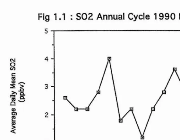
Observed concentrations of SO2 exhibit strong cyclic variation, on both a diurnal and annual level. These cycles are a result of various factors. The annual cycle for primary pollutants reflects the demand for energy throughout the year*, whereas the diurnal cycle depends more on meteorological and chemical factors (Fowler & Cape 1982). The cycles can be very site dependent, as a result of whatever sources are nearby. For example if examining the diurnal cycle from a site near to a road, peaks can often be observed at 'rush hour' times.

Annual cycle

For Europe, the cycle typically exhibits a maximum during the winter, reflecting the change in demand for energy (Fowler & Cape 1982). Figure 1.1 gives the annual cycle of SO2

levels observed at ITE Bush in 1990.

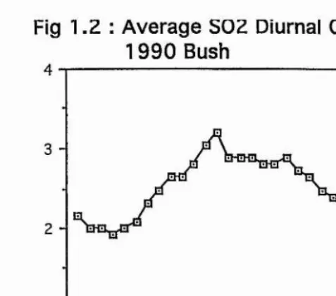
Diurnal cycle

The diurnal cycle of observed SO2 and NOx levels typically follow a very similar pattern to each other. The diurnal cycle is generated by a combination of factors, including rates of emissions, deposition rates and meteorological conditions (Fowler & Cape 1982). Figure

Fig 1.1 : S 0 2 Annual Cycle 1 9 9 0 Bush

cu

0

to

II

1

I

5

4

3

2

1

6 8 10 12

4 14

2

0

È

&

i

c

0) u

8

(\l

O (/)

Fig 1.Z : Average SOZ Diurnal Cycle

1 9 9 0 Bush

4

3

2

1

10 20

0 30

S02-Freauencv distribution

One method for summarising the behaviour of pollutant levels has been to ignore the time ordering of the observations and to fit a frequency distiibution to the set of all measurements of pollutant levels obtained over a certain period, often a year. This distribution summarises the behaviour of the pollutant over time, and can be used to estimate the frequency of occurrences of different pollutant levels. These frequencies can be used in conjunction with models for damage to plants, people or materials as a function of pollutant levels to estimate current levels of damage. Owing to the fact that the time structure of the data has been ignored, this approach at best merely provides a statistical description of pollutant levels and gives no understanding of the processes governing these. Despite this, such descriptions of the data can still prove useful, and often form the basis for air quality control legislation, pai'ticularly in North America (Smith, Fowler & Cape 1989). The use of a frequency distribution as a summary of pollutant concentrations is further complicated by the fact that data are obtained from a large network of different sites giving different types of

observations. Obseiwations may be given in the form of spot values at regularly spaced intervals, averages or maxima are also often recorded for eveiy 15 minutes, hour or whole day. The form of the data will affect the model used, for example methods constmcted with

The frequency distribution of observed SO2 concentrations (assumed to be averages over given time periods) can often be well described in the cential portion, say between the 20th and 95th percentiles, by a lognoimal distribution (Smith Fowler & Cape 1989). Much analysis follows the work of Lai'sen (1973, 1974), which is based on an empirical model for the data based on the following thiee properties:

• Frequency distribution tends to be lognoimal

• Median averaged concentration proportional to a power of length of averaging inteiwal.

• Maximum averaged concentiation proportional to an inverse power of length of averaging inteiwal.

This method allows for prediction of median and maximum values for a given averaging time if the data are available for another averaging time. For example, if daily mean values are available over a sufficiently long period of time (usually several years), then the hourly median and maximum and the annual median and maximum can be predicted. The design of air quality control legislation, especially in North America is frequently based on this

approach, as they aie often expressed in terms of average concentrations which should not be exceeded for more than one hour or one day per yeai\

1.4 : Secondary Pollutants:

Ozone is produced in polluted air by a complex series of photochemical reactions. The rate of these is lai’gely dependent on weather conditions and the levels of some other (primary) pollutants. There are also large reservoirs of ozone in the stratosphere which in certain weather conditions can be transported into the troposphere, leading to an increase in ground level ozone (PORG 1987).

Photochem ical Ozone Production

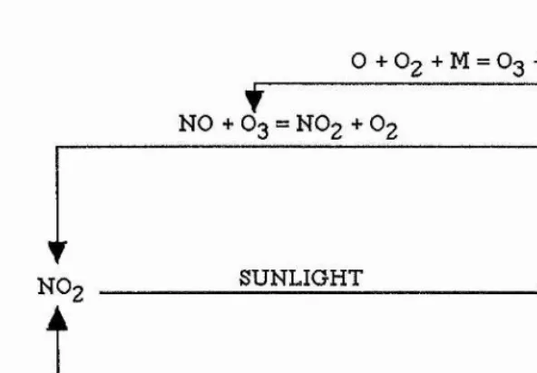
Ozone is foimed in the troposphere in a complex photochemical reaction with the by­

Figure 1.3 : Ozone photochemical reaction

M: Any molecule capable of dissipating the released energy eg. Nitrogen, Oxygen

O + + M = + M

NO + O') = NO-) + O

SUNLIGHT _{I^N O + O}

NO + V0CS">N02

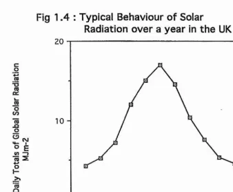
The amount of ozone resulting from this reaction is thus dependent on the levels of N 02 and VOCs present. As the reaction is driven by sunlight, the ozone level will also be weather dependent. There aie four main requirements on the weather for ozone formation (PORG

1993):

• Sunshine to drive the chemical reactions. • Low wind speeds to inhibit dispersion.

• Restricted boundary layer depths, to allow the build up of precursors (eg. NO2, NOx)

• Air temperature above 20®C to enhance evaporation of hydrocai'bon precursors and promote certain chemical reactions.

Fig 1

Typical Behaviour of Solar

Radiation over a year in th e UK

!

_ro

a

I

l é

f

1

20

10

-14

2 6 12

0 4 8 10

photochemical production over a year. As there is significantly more solai* radiation in the summer, so too there will be much more photochemical ozone production.

Ozone Depletion

Ozone is deposited readily onto vegetation and soil, in a process teimed diy deposition. The mechanism of deposition can be divided into two stages. Turbulent diffusion transports ozone to within a millimetre or two of the absorbing surface and then surface processes determine the mechanism of uptake. Rates of turbulent diffusion are determined primaiily by wind velocity and the aerodynamic roughness of the surface. For example the transport rate above a rough surface such as a forest will be greater than that over a smooth surface such as short grass. Another factor which affects the rate of turbulent diffusion is the vertical profile of air temperature; unstable conditions lead to larger rates of turbulent diffusion and vice versa. For vegetation, the most important terrestrial surface, uptake is primarily within the leaves following stomatal absoiption. As stomatal opening follows a marked diurnal cycle, with stomata opening in the morning and closing in the evening, so too does the deposition rate. This cycle does however often become obscured in the field owing to increases in atmospheric resistances at night.

Stratospheric Ozone

All atmospheric ozone is produced photochemically. Most is foimed in the stratosphere, giving rise to what is teimed the ozone layer. Usually there is little exchange between the stratosphere and the troposphere. However given the correct atmospheric conditions, intrusions of stratospheric air, rich in ozone, can enter the middle and lower troposphere as fai' as the atmospheric boundary layer. The weather conditions which lead to such

Annual Cvcle

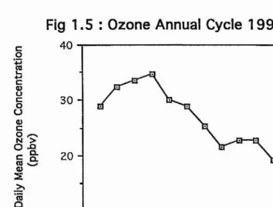
Due to the weather dependence of the processes affecting ozone production and depletion, with highest production occurring during the summer, ozone levels exhibit strong cyclic variations on a seasonal level. Typically, concentrations will peak during the spring, as a result of a similai' peak in stratosphere / troposphere exchange and an increase in the

frequency of days where photochemical production occurs. There is also typically a drop in levels during August / September as the frequency of days in which photochemical

production occurs is reduced.

The annual cycle of ozone levels for ITE Bush in 1990 is illustrated in figure 1.5. This follows the typical pattern described above.

Diurnal cvcle

Fig 1.5 : Ozone Annual Cycle 1 9 9 0 Bush

40

30

-O

II

-CD

ra 0 2 6

Month

10

1.5 : Effects Of Air Pollutants

Effects Of Ozone

Modelling Pollutant Damage

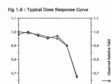
The most comprehensive study carried out to date has been in North America by NCLAN (the National Crop Loss Assessment Network) which was begun in 1980 to develop an understanding of the effects of pollutants (primarily ozone) on agricultural crops. They have studied crops growing in open topped chambers, exposed to controlled amounts of pollutants. Some work has been carried out by growing crops in ambient levels of

pollutants and comparing the yield obtained against that of crops growing in chambers with the pollutants removed. This approach is useful only for assessing damage due to current levels of pollution, but a study using widely vaiying levels of pollutants will be more useful for modelling purposes. This approach allows the plant damage to be linked by some function to the pollutant dose and allows assessment of possible future damage under many different scenarios and calculation of economic and environmental gains for given

reductions in pollutant levels. However, such experiments are difficult to construct well, and ideally are conducted over a long period of time. In addition the temi 'pollutant dose' has to be caiefully defined. Many possibilities exist, for example daily mean concentrations or time spent above a thieshold level. The best modelling approach depends on the

mechanisms which govern damage in a paiticulai’ situation, however there are many gaps in knowledge of these.

Fig 1.6 : Typical D ose R esponse Curve

u.

I

LL

0.9 - 0.9

0.8 - - 0.8

0 .7 - - 0 . 7

0.6 0.6

0.10 0.15

0.00 0.05

I

Weibull Function Fit Observed Relative Ye!

Chapter 2: SOo : Frequency distribution

2.1: Introduction

The usual analysis of data from monitoring of pollutant gases assumes that the frequency distribution of obsei*ved concentrations can be described by a lognormal distribution (Smith, Fowler & Cape 1989), (Fowler & Cape 1982).

However, the fit of the lognormal distribution in the upper tail of the distribution is poor, with the lognormal under-predicting the frequency of higher concentr ations (Smith, Fowler & Cape 1989). As damage occurs mainly at these higher concentrations, this under­

prediction gives rise to concern over the use of the lognormal based approach to legislate air quality standards.

The inverse Gaussian distribution has been suggested as a possible alternative to the lognormal distribution for the frequency distribution of SO2 levels. The upper tail of the inverse Gaussian is heavier than that of the lognormal and may be able to improve this lack of fit to the data.

2.2: Methods

The Inverse Gaussian distribution has the probability density firnction (Chhikar*a & Folks 1989):

i t X exp

f

2p2x x> 0 (2.1)

The maximum likelihood estimators mle(p) and mle(%) of p, and

X

mle(p) = X

(2 .2 )

mle(À)

(2.3)

Both the inverse Gaussian and 2 par ameter lognormal distributions have been fitted by maximum likelihood to a data set consisting of 15 minute averages of SO2 concentr ations (ppbv) at ground level at ITE Bush over 1990. This data set contains 33371 observations, with 1667 missing observations spread randomly throughout the year.

Two standard tests were used to assess the fit of both distributions: the Kolmogorov- Smirnov test, and the Cramer-VonMises test.

been used. This test is appropriate given the importance of the fit of the disti ibution to the upper tail in this case.

This test statistic is calculated by the formula:

AUn2 = | - 2 % F (x (j) ) - ] 2 [2 ' l° g [l ' (2-4)

j= l j= l

2.3: Results

The parameters of the inverse Gaussian distribution were estimated by maximum likelihood. The estimates were p=2.5440 and X;=1.3118.

The 2 parameter lognormal distribution was also fitted. The parameters were estimated as p=0.4890 and 0=0.96753.

The values of the thiee test statistics were calculated for both distributions. The results are summarised in table 2.1:

Table 2.1 : Values of lack of fit test statistics

Test Lognormal Inverse Gaussian Critical Value Kolmogorov-Smirnov: D 0.043 0.133 0.007 Cramer-VonMises: T 18.89 199.04 0.461 Mod Anderson-Darling: AUn^ 41.27 351.37 0.432

Table 2.1 indicates that the inverse Gaussian does not fit the data as well as the lognormal. In addition, the values of indicate that the lognqrmal fits the upper tail considerably more accurately. The results confirm that the lognormal does not fit the data particularly well, as the values of all three test statistics are greater than their critical values.

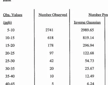
The behaviour of the distributions in the upper tail of the distribution has been mentioned to be of interest. To investigate this further, table 2.2 summai'ises the behaviour of

Table 2.2: Number of observations recorded an d predicted ab o v e 5

p p b

Obs. Values Number Obseived Number Predicted

(ppb) Inverse Gaussian Lognormal

5-10 2741 2989.65 3103.25

10-15 618 819.14 651.61

15-20 178 296.94 204.31

20-25 97 122.68 79.99

25-30 42 54.73 36.16

30-35 20 25.67 18.10

35-40 10 12.49 9.78

40-45 5 6.24 5.61

45-50 1 3.18 3.38

>50 4 3.54 6.67

2.4: Conclusion

The work carried out in this chapter has confirmed that the lognormal distribution does not fit the frequency distribution of observed SO2 concentrations from ITE Bush in 1990 particularly well.

Chapter 3: Modelling Instrumental

Variation

3.1: Introduction

In many envii'onmental studies today, data aie obtained automatically by instruments recording 'continuously', which may mean either point readings at frequent time intervals, or aggregated levels over short time periods. This can lead to an overwhelming volume of data if the observations continue over long periods. Frequently, because of this, the values recorded may be at longer time intervals, with perhaps as many as 100 consecutive

observations taken and summarised as an average or summed value and then recorded.

With instruments recording in this manner, the calibration may change over the time periods considered. Ideally, the instmment will have been recalibrated at regular* intervals, leaving a gap in the recorded data. The data between successive calibration times may then have been adjusted by a linear* transfoi*mation to compensate for the instr umental drift obseived.

The 'raw data' made available for analysis are the end results of these processes.

Another problem that can occur with data of this type is the presence of outliers caused by a sudden change in the recorded values for only one or two consecutive observations.

3.2: Methods

The data analysed in this chapter aie measurements on levels of ground level ozone, measured in par ts per billion (ppb), at ITE, Bush Estate, Midlothian, as a small part of a much wider project studying ozone levels (Fowler & Cape (1982) and Smith, Fowler & Cape (1989)). This data set is unusual in that readings are available from two separate instruments, which aie operating over different time spans. One (M L03) is present more or less continuously, and the other (AA03) is present when not required for fieldwork

elsewhere. This provides the opportunity to study the differences between the readings on the two instruments. According to the manufacturer's specifications, these are said to have slightly different characteristics, the AA03 having better accuracy at low levels of ozone, and a lower detection limit. The M L03 gives readings every 12 seconds, and the AA03 every 7 seconds, but for both machines the data provided are averages over 15 minutes of the higher frequency records.

3.3: Results

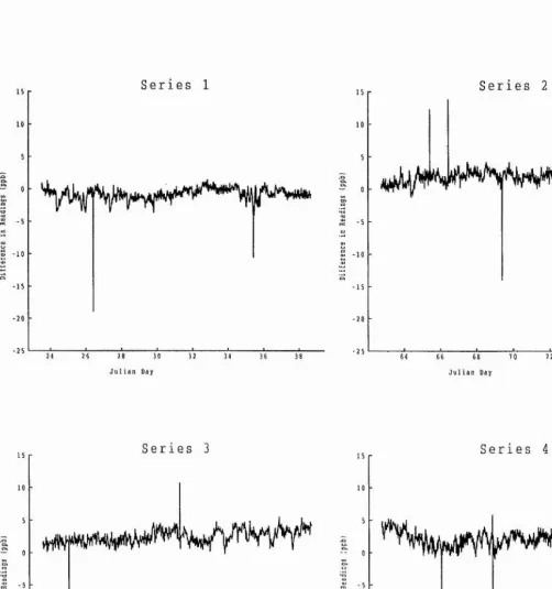
In fig. 3.1 the differences between the 2 readings aie plotted as a time series. These plots highlight a problem in this data set with outliers. The spikes that can be seen in the time series plots are caused by the reading from one machine 'jumping' up for one reading and then returning to its previous level. Both analysers exhibit this behaviour with roughly the same frequency. These spikes are thought to be a feature of the data recording device, and not true observations on ozone levels for the following reasons:

1. The 'jump' occurs on only one of the two machines at any one time. If there had been an actual increase in ozone levels over even such a short time span, one would expect both machines to have recorded it.

2. An examination of data for other gases present (nitrogen oxides, sulphur dioxide) did not indicate that an increase in ozone levels had occurred as the level of ozone observed is linked to levels of other gases present in the atmosphere. If the spike were a true observation, one would expect a corresponding spike to occur in the records for the other gases at the same time. For details of the interactions between different pollutants see Fowler & Cape (1982) and Smith, Fowler & Cape (1989).

For the remainder of this work, these spikes were treated as missing observations and were replaced using a simple average of the observations immediately before and after the spike.

A spike at time t on machine 1 has been replaced by the value:

(X 1,1-1 - X2,t-i) + (X j't+ l ~ X2,t+l)

2

Fig 3.1: D ifferences between readings on ozone analysers

S e r i e s 1 S e r i e s 2

%

I

- 10 -1 0

- 1 5 - 1 5

- 2 0 - 2 0

- 2 5 - 2 5

J u l i a n Da y J u l i a n Da y

S e r i e s 3 S e r i e s 4

- 1 0 - 1 0

- 1 5

- 2 0

- 2 5

1 0 0 1 0 2 . 5 1 05 110 1 1 2 . 5

3.4: Time Series Analysis of Differences

Model Selection

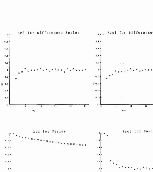
The autocorrelation and partial autoconelation sequences for the data were calculated (with the spikes removed), these are shown in figs 3.2-3.S. The PACF decays to near zero after lag 1 or 2 while the ACF shows a more gradual decay. After differencing the series once, both the ACF and PACF exhibit a rapid decay after lag 1 or 2. Plots of the data after differencing show no obvious trends in level or variability, implying stationaiity. There are also no obvious short or long term seasonal effects. These facts point to the use of one of three different Box-Jenkins type models (Wei 1990), which are described below:

l.IM A (l,l);

Zj; = + a^; - MA(1) aj;_]^ -(1 )

(where Z^ is the difference at time t, and a^ is a random shock at time t)

2. IMA(1,2):

Zt = Zj_j + a^ - MA(1) - MA(2) a^_2 -(2 )

3. ARIMA(1,1,1):

=AR(1)W^_1 + a^ - MA(1) a^_i -(3 .1 ) where

Fig 3.2: ACF and PACF for series 1, before and after differencing

Ac f f o r D i f f e r e n c e d S e r i e s

0 . 2

X v X X X

V X X X X

10

La g

0 . 4

0 . 2

-0 . 2 -0 . 4

P a c f f o r D i f f e r e n c e d S e r i e s

X X X x X ^ X X x * X * x X X X X X * X

La g

1

0 .(

0 . 2

-0 . 2

-0 . 4

•0.»

Ac f f o r S e r i e s

X X X X X X X X _{X X X X X}

0 5 10 15 20 25

Lag

0 . 4

- 0 . 1

P a c f f o r S e r i e s

X X X * X ^ X ^ x X ^ X x X x x

Fig 3.3: ACF and PACF for series 2, before and after differencing

o.s

0 . 4

0 . 2

■0 . 6

Ac f f o r D i f f e r e n c e d S e r i e s

X ^ X x x X x X ^ X x

La g

25

1 r A, P a c f f o r D i f f e r e n c e d S e r i e s

0 . 4

0 . 2

1-0 . 4

- 0 . 1

-1

X X X X X X X X X X X X X X

Lag

1 5 2 5

Ac f f o r S e r i e s P a c f f o r S e r i e s

XXX

0 . 0

o . t

0 , 4

0 .2

0

- 0 . 2

-0 . 4

X X X X X X X X X X X X X

-0.0

lag

Fig 3.4: ACF and PACF for series 3, before and after differencing

Ac f f o r D i f f e r e n c e d S e r i e s

Lag

A c f f o r S e r i e s

La g

P a c f f o r D i f f e r e n c e d S e r i e s 1

0 . 1

0.(

0 . 4

0 . 2

0

0 . 2

0 . 4

0.(

0 . 1

1

0 . 4

P a c f f o r S e r i e s

5 10

Fig 3.5; ACF and PACF for series 4, before and after differencing

A c f f o r D i f f e r e n c e d S e r i e s

o . t

o . t

-0 . 2

-0 . 6

- O . t

Lag

2 5

P a c f f o r D i f f e r e n c e d S e r i e s

0 . 4

-0 . 2

- O . t

La g

1

0 . 6

Ac f f o r S e r i e s

X X

X X _{X X}

X X

X X X X X

P a c f f o r S e r i e s

0 . 4

x ^ x x x x ^ * x _ x x x X^ x

-0 . 2

-0 , 6 -0 . 6

20 25

Model Fitting

Table 3.1 contains the estimates of the pai*ameters for each of the three models indicated as possibilities above for the four data sets considered here, both with the spikes present and removed. The t-ratio also quoted is an indication of whether or not the parameter is required in the model, with a low t-ratio leading to the conclusion that the term with that parameter should not be included. For details see Wei (1990).

TABLE 3.1 - Estimates of param eters an d t-ratios

IMA(1,1) IMA(1,2)

Series MAI t-ratio MAI t-ratio MA2 t-ratio ARl t-ratio MAI t-ratio

1 no spikes 0.40 16.83 0.39 14.71 0.06 2.26 0.18 2.97 0.56 10.96

1 spikes 0.63 31.24 0.60 22.89 0.07 2.54 0.12 2.89 0.71 25.22 2 no spikes 0.45 19.06 0.40 15.28 0.12 4.52 0.27 5.15 0.67 16.85 2 spikes 0.80 51.31 0.77 28.91 0.06 2.07 0.08 2.42 0.84 48.91 3 no spikes 0.30 10.12 0.27 9.17 0.23 7.80 0.69 26.65 0.94 87.50 3 spikes 0.89 67.54 0.84 28.54 0.07 2.43 0.09 2.91 0.92 76.41 4 no spikes 0.38 18.17 0.34 15.26 0.14 6.18 0.36 7.76 0.04 19.47 4 spikes 0.73 47.79 0.73 32.19 0.01 0.27 0.01 0.30 0.74 35.66

ARIMA(1,1,1)

For all of the data sets used, both with and without spikes, the first MA parameter is seen to be higlily significant, whilst the second MA paiameter is just significant with the spikes removed, and less significant in all cases with the spikes present. The AR parameter is also just significant when applied, except for series 3 with the spikes removed, when it is highly

Table 3.2 contains the values of a test of normality applied to the residuals from each of the models essentially equivalent to the Shapiro Wilk test, based on the correlation of the data and their 'normal scores' - for details see Filliben (1975). The critical value for this test for n=100 is 0.994. The value of this test statistic does not change significantly across the three models considered, but does across different data sets. The residuals from the models fitted to the data sets with the spikes not removed can definitely not be regarded as normally distributed, whilst with the spikes removed only the residuals from data sets 1 and 4 aie questionably normal. Normal probability plots and histograms of these residuals suggest that they come from a symmetric distribution, with slightly heavier tails than the normal.

TABLE 3.2 - Test of normality on residuals

Number of Series IMA(1,1) IMA(1,2) ARIMA (1,1,1) observations

1 no spikes 0.992 0.991 0.991 1456 I spikes 0.750 0.748 0.74 1456 2 no spikes 0.998 0.998 0.998 1414 2 spikes 0.690 0.686 0.685 1414 3 no spikes 0.998 0.997 0.998 1123 3 spikes 0.571 0.564 0.562 1123 4 no spikes 0.991 0.992 0.992 1954 4 spikes 0.711 0.710 0.710 1954

TABLE 3.3 - SS an d MS residual after model fitting

Series IMA(1,1) IMA(1,2) ARIMA (1,1,1)

SS MS SS MS SS MS

1 no spikes 315.83 0.22 314.79 0.22 314.55 0.22 1 spikes 811.39 0.56 808.28 0.56 808.01 0.56 2 no spikes 455.23 0.32 449.28 0.32 449.16 0.32 2 spikes 2385.03 1.69 2378.39 1.69 2377.65 1.69 3 no spikes 339.43 0.30 323.29 0.29 317.35 0.28 3 spikes 2680.61 2.39 2666.0 2.38 2664.41 2.38 4 no spikes 526.38 0.27 516.13 0.27 514.69 0.26 4 spikes 1786.04 0.91 1785.97 0.92 1785.97 0.92

The ACF and PACF sequences for the residuals from each of the models fitted were also examined, and no significant autocorrelation structure was observed.

3.5: Discussion

The IMA( 1,1) model;

Zt = Zt_i + at - MA(1) at-i

(where Zt is the difference at time t, and at is a random shock at time t)

would be an intuitively reasonable model for the series. To see this, write the model for the Z's explicitly as a function of past and present a-values:

Zt = at + (l-6)at_i + (l-0)at_2 + . . . + (l-9)a_jji - 0a-m -l

where -m is earlier than time t= l, at which point we first observed the time series, and 0 is the MA(1) par ameter in the model. Since we are assuming that -m<l and 0<t, we may usefully think of Zt as being an equally weighted accumulation of a lar ge number of white noise values.

In terms of the ozone analysers, if we regard each white noise value as being the random drift in calibration between the two machines during the fifteen minute period, the value of Zt being an accumulation of these would seem to be a reasonable model for the data (i.e. a sum of all these random drifts since the analysers were turned on together).

The theory of temporal aggregation of the ARIMA process (Wei 1990) states that if a disaggregated series (denoted by z^) is aggregated to form the series Z^, the m-period nonoverlapping aggregates of z^, by summing every m successive z^'s, then the following results hold:

1. If Zt follows an IMA(d,q) model, then Z^ follows an IMA(d,No) model, where Nq is defined by:

NQ< q* = [d+l+(q-d-l)/m],

and [x] is used to denote the integer part of x.

2. If Zt follows an ARIMA(p,d,q) model, then as m -> oo , the limiting model for the aggregates Zt exists and is the IMA(d,d) process, independent of p and q. A similar result holds if the disaggregate series follows a seasonal ARIMA(p,d,q)x(P,D,Q)s model, leading to an IMA(D+d,D+d) process.

These results give a possible justification for selecting the IMA(1,1) model for the data as follows:

The data given are aggregates of a lar ge number of observations, with m being equal to 75 for the M L03 data and 129 for the AA03 data.

possible models for the disaggregated series lead to an IMA(1,1) model as a model for the aggregates.

Unfortunately, only a very small amount of data from the disaggregated series is available, and if some can be obtained some useful work in this direction could be done.

3.6: Conclusion

The work outlined in this chapter indicates that one of the models considered may prove useful when analysing data of this type. Although the lack of fit of the model could be improved by either transforming the data in some way to induce noimality, as the coiTelation structure appears to be well modelled, or using an IMA type model with a non-gaussian random shock distribution. Also, a study of the disaggregated series could prove highly useful in finding the type of model required.

The spikes observed in the data are also thought to be highly important, for two reasons:

First, it is seen that the analysis described in this chapter is affected if the spikes are ignored, the choice of model for a particular* data set may change, and the fit of the model is also very much affected.

Chapter 4: Modelling Monthly Average

Ozone Curves

4.1: Introduction

A common feature of analyses of ozone monitoring data is the average diurnal cycle. This average cycle is calculated either as the average over a year or, in some cases, as the average over a few months. For example, in the PORG interim report (1987), a variety of diurnal cycles aie displayed. Some are the averages over April to September, some aie averages over a whole year, and one figure displays the six cycles for the months July to December sepaiately. However, the only discussion of how the cycle varies over a year is a statement that there is generally a more pronounced diurnal cycle observed in the summer.

It is known that observed ozone levels depend largely on the weather (PORG 1987 & 1993) and that the distribution of weather types varies over a year*. These facts should lead to changes in the diurnal behaviour of ozone at different times of the year*. This chapter will investigate the variation in the average diurnal cycle over a year.

4.2: Methods

The data analysed in this chapter are measurements on levels of ground level ozone, measured in paits per billion (ppbv), at ITE, Bush Estate, Midlothian during 1988. The 'raw data' are the 15 minute averages from the M L03 machine considered in the previous chapter, with all the known 'spikes' removed.

To calculate the average diurnal cycle over a specific period, all the obseiwations available at each of the 96 15 minute time points in a day have been averaged sepaiately:

If Oij represents the ozone level at time j in day i, (i=l...N , j=1...96), the level of the average cuiwe for these N days at time j, Aj is calculated as:

i-S

Aj “ N i=l

The average diurnal cycle for the whole of 1988 is shown in fig 4.1. The average diurnal cycles for each of the twelve months of 1988 aie shown in fig 4.2.

Fig 4.1: Bush 1988 A v e r a g e Ozone d iurnal curve

45

40

35

30

25

20

15

0 5 10 15 20

Fig

4.2

(part 1): Monthly average ozone diurnal cycles for 1988

J a n , F e b , Mar

50

45

40

35

30

25

20

15 ₀

10

5 15 2 0

Jan V time

Feb V time Mar V time

T i m e o f d a y ( h o u r s )

A p r , Ma y , Jun

50

45

35

30

2 0

15 _{0 5 10 15 20}

Apr V time May V time Jun V time

Fig 4.2 (part 2): Monthly average ozone diurnal cycles for 1988

J u l , A u g , Sep

50

45

40

35

30

25

20

15 _{0 5}

10 15 20

Jul V time Aug V time Sep V time

T i m e o f d a y I h o u r s I

O c t , N o v , D e c

50

40

35

30

25

2 0

15 _{C 5 10 15}

20

Oct V time Nov V time Dec V time

Time Distortion

Fig 4.2 demonstrates that the diurnal cycles have differing shapes for each of the twelve months. They all have a 'hump' starting at between 5 and 8 am and finishing between 4 and

8 pm. This section of the curve represents the daytime vaiiation in ozone levels and is driven by a combination of factors including sunlight, temperature and wind speed. These factors depend more on the position of the sun in the sky than clock time. This suggests using the time of day relative to the sun and not clock time as the time used on the x-axis.

To do this a transformation of the time axis is required for each day of the year (thanks to C.D.Steele for help with this transformation) which is caiTied out as follows:

1. For each day of the year where observations aie available calculate declination of the sun, 6, using the following equation:

sin 8 = sin e sin _365.25 8=23.45°

d=days since March 21^1

2. Once this has been caiiied out, use the value of 5 to calculate transformed times t' for each time point t during that day where an obseiwation is given. For each time point t calculate transformed times t' as follows:

From the time t, in hours, calculate angular time A (degrees):

A =15*t t=time in hours

Then calculate the transformed angular time A using the following equation:

-cos (i> sin A J. , tan A = Where (j) = latitude.

sin ()) tan ô - cos (j) cos A

The transformed time in hours t' is then given by:

t'=A'/15

The transformed times t' have been calculated for eveiy time point t at which an ozone reading is available. This results in a set of daily ozone curves plotted on a time axis where sunrise, sunset, midday and midnight occur at the same transfoiined time for every day of the year.

maximum change in ozone levels between two successive 15 minute time points is small (97% of such changes are less than 4ppb in the data set used here).

Fig 4.3 (part 1): Monthly average diurnal cycles (Transformed time)

J a n , F e b , Mar

50

45

40

35

30

25

20

15 _{0 5 10 15 2 0}

Jan V time Feb V time Mar V time

T r a n s f o r m e d T i m e

A p r , Ma y , Jun

50

45

40

35

30

2 0

15 _{0 5 10 15 20}

Apr V t i m e

May V t i m e

Jun V t i m e

Fig 4.3 (part 2): Monthly average diurnal cycles (Transformed time)

J u l , A u g , Sep

50

45

40

35

30

25

20

0 5 10 15 2 0

Jul V time Aug V time Sep V time

T r a n s f o r m e d T i m e

O c t , N o v , Dec

50

45

40

35

30

25

2 0

15 _{0 5 10 15 20}

Oct V time Nov V time Dec V time

4.3: Model For Ozone Curves

Fig 4.4 shows the same curves as fig 4.3, calculated with the start of each day at 7am on the transformed time axis. 7am transformed time corresponds to l/24th of the daytime after sunrise. This is when one expects the daytime processes to begin affecting the observed ozone concentration as it will on average take approximately an hour for the night time inversion layer to break up.

The curves plotted this way naturally divide into two sections, representing the daytime and night time variation of ozone separately. Both the daytime and night time sections exhibit variation in spread and level, but the shapes remain very similar from month to month. A model for these data will have to be capable of reproducing this variation in spread and level separately for both sections of the day.

Day and night sections have been modelled separ ately as polynomials in time of the fifth degree. These have been constrained to be continuous in value and first derivative at the join between day and night (at the centre of the time axis) and at the beginning and end of

Fig 4.4 (part 1); Monthly average diurnal cycles

(Shifted transformed time)

J a n , F e b , Mar

50

45

40

35

30

25

2 0

15 _{0 5 10 15 20}

Jan V time

Feb V time

Mar V time

S h i f t e d T r a n s f o r m e d T i m e

A p r , Ma y , Jun

50

45

40

35

30

25

2 0

15 _{0 5 1 0 15 20}

Apr V time Hay V time Jun V time

Fig 4.4 (part 2): Monthly average diurnal cycles

(Shifted transformed time)

J u l , A u g , Sep

50

45

40

35

30

25

2 0

15 _{0 5 10 20}

Jul V time

Aug V time Sep V time

S h i f t e d T r a n s f o r m e d T i m e

O c t , N o v , Dec

50

40

35

30

25

2 0

15

Oct V time Nov V time

Dec V time

For algebraic simplicity use - l < x < + l a s x variable, -1 is 7 am transformed time, and +1 is 7am transformed time the next day. The model can be written as:

Where Ql(x), Q2(x) aie polynomials of the fifth degree in x with constraints:

Qi(-1) = Q 2(+ 1);Qi(0) = Q2(0)

Q i’(-I) = Q2’(+1) ; Qi'(O) = Q2’(0)

Each quintic has six coefficients, twelve in all for each month. The continuity conditions impose four constraints on these, leaving a total of eight independent pai ameters for each of the twelve monthly curves. The model will thus reduce to a series of lineai* combinations of eight polynomial functions of x. When the constraints are implemented the model reduces to:

8

E[yij]= S ®ki fkj i=1...12, j=1...96 k=l

Where:

yij: obs in month i, time point j. Time x = -1+2/96 * (j-1)

fkj: polynomials fk in x at time point j.

The polynomials % aie determined by the constiaints imposed and aie given by;

fl = l f2 = (x3 - x)

f3 = (x4 - 2x2)

f4 = (x^ - x)

f5 = ((x+)2 - 0.5x - 0.5x2) f6 = ((x+)^ “ 0.5x - 0.75x2)

t ]

fg = ((x+)5 - 0.5x - 1.25x2)

Where (x+)H = | ” n ^ > 0

This model can be fitted directly to the data, using a least squares algorithm. The paiameters aie the Gjô, eight for each of the twelve monthly curves. Thus this model requires a total of 96 paiameters to model the whole year's monthly vaiiation.

Fig 4.5 shows the twelve curves generated by this model, with the actual data points plotted for compaiison. This model fits the monthly averages well. To allow comparison with other modelling approaches that will be considered later, the lack of fit of the model has been assessed by calculating the area between the cuiwe generated by the model for each month and the data cui*ve. Using aiea between two curves as a measure of the distance between them has vaiious advantages over most standard measures as is discussed in

Fig 4.5 (part 1): Fit by 8 parameter 2-Qmntic model

raw data xxxx model fit

J a n Feb

Mar Apr May

Fig 4.5 (part 2): Fit by 8 parameter 2-Quintic model

raw data xxxx m odel fit

Oct Sep

T

able 4.1 : Lack of fit (area betw een curves') for 6 modelling ap p ro ach es

Jan Feb Mar Apr May Jun Jul Aug Sep 96 Par (Fig 4.5) 42.1 27.1 36.1 71.4 50.9 39.5 37.8 26.5 42.0

2 Corr PC (Fig 4.9) 89.2 216.5 60.5 243.3 935.2 379.1 107.3 223.3 183.6

3 Corr PC (Fig 4 .n ) 102.0 226.7 55.7 139.7 749.9 535.1 125.1 139.8 97.0 2 Cov PC (Fig 4.14) 2407 2541 2518 2299 3502 2287 2689 2535 2367 4 Cov PC (Fig 4.16) 2640 2591 2717 2636 3639 2469 2870 2701 2466 40 Par (Fig 4.19) 78.0 45.9 51.4 79.0 58.2 68.8 79.1 61.8 58.2

Oct Nov Dœ Averac;e 96 Par (Fig 4.5) 42.7 91.4 24.9 44.4

2 Corr PC (Fig 4.9) 234.2 135.2 217.3 252.0

3 Corr PC (Fig 4.11) 92.0 178.3 43.8 207.2 2 Cov PC (Fig 4.14) 2221 2599 2784 2546 4 Cov PC (Fig 4.16) 2397 2825 2921 2739

4.4:

Parameter Reduction

Fig 4.6 shows the estimates of each of the eight paiameters of the 2-quintic model over the twelve months of 1988. The parameters exhibit only 2 basic patterns: 06 and Bg show the same pattern, 65 and 87 show the inverse pattern to 02, 03 and 04, and 0i shows a similai pattern to 05 and 07. Because of this it may be possible to reduce the number of parameters in the model from eight to two or three for each month.

Using two parameters per month, say \j/i and Çi (i=1...12), estimates for 0i,...,0g can be calculated as linear combinations of these new parameters by using a function of the form:

0ki = akV i + Pk^i (k=1...8)

This will reduce the number of parameters required to model a year from 96 to 40.

Estimates of \}/i and will be required for each of the twelve months (total 24 parameters), and estimates of the eight a k and Pk (total 16) will also be required.

Two possible approaches for obtaining estimates of \j/i, Çi, a k and pk will be considered. The first method will be to use a principal components procedure on the original estimates of

Fig 4.6: Estimates of 8 parameters in the 2-Quintic model

Par 2 Par 1

Par Par 4

Par 3

Par Par 1

F

irst M ethod

To obtain estimates of y i, ajc and pk from a principal components analysis of the estimates of the 0ki the following approach was adopted:

The principal components analysis gives the value of each principal component as a linear’ combination of the eight parameters:

PCmi ~ hm(^li>'**»6 8i) m =1...8 , i=1...12

(where PCmi is the value of principal component m in month i)

If we set the last 6 principal components equal to zero (say), we obtain a set of simultaneous equations which can be solved to obtain each of the 9ki as functions of the values of the first

2 principal components.

Thus:

set PCmi = 0 m=3...8 (say) , i=1...12

gives the set of equations:

P C ii = h i(eii,...,0 8 i) PC2i = h2(eii,...,08i)

0 = hm(01i,...,08i) m=3...8

which can be solved simultaneously to give the result:

This result allows calculation of estimates for the eight model parameters from the values of PCi and PC2 obtained from the principal components analysis. By changing the number of PC's set to zero at the start of this procedure, it is possible to obtain estimates as functions of any number of the principal component scores, allowing flexibility in the number of parameters used for each month.

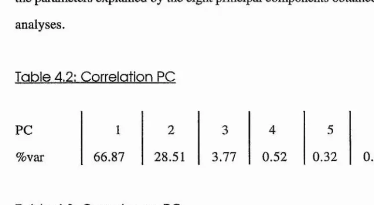
To this end, principal components analyses using both the correlation and covariance matrices were carried out on the parameter estimates. Both types of principal components analyses have been carried out as there is no obvious justification for being interested primarily in the shape or level of the par ameters. This is because the primary aim of this procedure is not to model the parameters, but to obtain estimates of the parameters which will then be used to model the data. Tables 2 and 3 show the percentage variation amongst the par ameters explained by the eight principal components obtained from both these analyses.

Table 4.2: Correlation PC

PC %var

1 2 3 4 5 6 7 8

66.87 28.51 3.77 0.52 0.32 0.01 0 0

Table 4.3: C ovariance PC

PC 1 2 3 4 5 6 7

%var 83.55 16.14 0.18 0.14 0 .00 0 .00 0

0

Fig 4.7 shows that the first two correlation PCs follow the two basic patterns observed in the parameters. Fig 4.8 allows comparison of the estimates for 0l,.,.,08 calculated using the above principal components method and their original estimates. The original parameter estimates are closely approximated. 0 i is the par ameter least well approximated. As fi= l,

01 represents the actual ozone level at x = 0 , or 7pm, and is added to the predicted ozone values at all other times. This will lead to an error in the level taken by the model.

Fig 4.9 shows that the ozone curves generated by this approach do not fit the data well when compared to the original model, especially for the months of May and June. This is confirmed by the lack of fit results displayed in table 4.1. The average lack of fit for this approach is over 5 times greater than that for the original model. There is a slight error in the level of the model values for many of the months, due to the error in 0i, and the model has failed to reproduce the correct shapes for many of the monthly curves.

To investigate if the lack of fit can be improved by including the third coiTelation principal component, estimates of 0i,...,0g were calculated as functions of the first three correlation principal component scores. Fig 4.10 allows comparison of these estimates and the

originals. This method provides more accurate estimates of 0i,...,0g, especially 0 i. Fig 4.11 shows that despite this improvement in the estimates of the parameters the inclusion of the third principal component has not greatly improved the fit of the model to the data. This is confirmed by the lack of fit results displayed in table 1, there has been a slight drop in the average lack of fit, but it is very small compar ed to the difference between these two

coiTelation PC approaches and the original approach. There has been a slight improvement in the fit for some months but the noted discrepancies for the months of May and June still exist.

Moving on to the covariance analysis, the first two PC's account for 99.69% of the

Fig 4.7: Values of correlation PCs

PC 1 PC 2

t

o.s

0

■0,5

1 . 5

•Î

Î . 5

2

1. 5

1

0 . 5

0

0 . 5

1. 5

10 12

i !

2 (

PC 3

1 . 5

I

0 , 5

0

0 . 5

Fig 4.8: Estimates of 8]^-8g as f(PCl,PC2)

original estimates f(PC l,PC 2)

Par 1 Par 2

Par 3

Par 6

Par 4 Par

Fig 4.9(part 1): Fit by first 2 correlation PC approach

raw data xxxx m odel fit

Jan

Mar

Jun

Feb

Apr

Jul

May

Fig 4.9(part 2): Fit by first 2 correlation PC approach

raw data xxxx model fit

Sep

Nov

Oct

Fig 4.10: Estimates of 0x"®8 ^ f(PCl,PC2,PC3)

original estim ates f(PC l,PC 2,PC 3)

Par 1 Par 2

Par 3 Par P a r 5

Fig 4.11 (part 1): Fit by first 3 correlation PC approach

raw data xxxx m odel fit

Jan Feb

Mar

Jun

Apr

Jul

Hay

Fig 4.11 (part 2): Fit by first 3 correlation PC approach

raw data xxxx m odel fit

Sep Oct

it is necessary to include the third and fourth PC's as they both make a veiy similar

contribution to the percentage variance explained and the contribution made by PC's 5,.„,8 are zero to 2 decimal places. If the third and fourth PC's aie included, the percentage variance explained increases to almost 100%.

Fig 4.12 shows that the first two covariance PCs also follow the two basic patterns observed in 01,...,08. Fig 4.13 allows comparison of the estimates for 0i,...,0g calculated using the first two covariance PC's and the original estimates. The original parameter estimates are less well approximated than by both the correlation PC methods. The discrepancy for 0% has now been greatly increased, as the use of the covariance matrix has reduced its importance to the analysis due to its small magnitude relative to the other seven parameters. 0y is now very well approximated, as it is by far the greatest in magnitude and as such has the highest importance to a covariance PC analysis. Fig 4.14 shows that the fit of the model to the data is extremely poor, there being now an error of approximately 30 ppb in the level of the curves generated by the model. As discussed above this is a result of a similar" error in the level of the estimates for 0 i. This is reflected in the lack of fit results in table 4.1, the average now being an order of magnitude greater than the two correlation PC approaches.

Fig 4.15 shows estimates for 0i,...,0g calculated as functions of the first four covariance principal component scores. These estimates are closer to the originals, except for 0%, which still exhibits a large error in level. Fig 4.16 confirms that this error in the level of 0i leads to a similar error in the level of the model fit, although except for the month of May, the shape of the fit is good. The average lack of fit is now even greater than the two covariance PC approach.

Fig 4.12: Values of covariance PCs

•100

no

PC 2

PC 3 PC 4

189

169

UO

199

39

69

29

9

3 19 12

6

Fig 4.13: Estimates of Oj-Og as f(PCl,PC2)

original estimates f(PC l,PC 2)

Par 1 Par 2

Par 3 Par Par 5

Fig 4.14 (part 1): Fit by first 2 covariance PC approach

raw data xxxx m odel fit

Jan

Mar

Jun

Feb

Apr

Jul

4 i 14 n 20

Kay

... ...

Fig 4.14 (part 2): Fit by first 2 covariance PC approach

raw data xxxx m odel fit

Sep

Nov

Oct

Fig 4,15: Estimates of G^-Gg as f(PCl,PC2,PC3,PC4)

original estim ates f(PCl,PC2,PC3,PC4)

Par 1 Par 2

Par 3 Par 4 Par 5

Fig 4.16 (part 1): Fit by first 4 covariance PC approach

raw data xxxx m odel fit

J a n Feb

g ; 10 o 20

Mar

Jun

Apr

Jul

Hay

Fig 4.16 (part 2): Fit by first 4 covariance PC approach

raw data xxxx model fit

Sep

Nov

Oct

Second M ethod

An alternative method is to reduce the dimensionality of the original 2-quintic model directly. In

8

Eiyij] = 2 0ki fkj i=1...12 , j=1...96 , k = l.,.8

k= l

write each 0]q as a linear combination of two new parameters, and as follows:

8

E[yij] = Z (^k¥i + Pk^i)

k=l

Vi s Kkfkj + s Pkfkj k= l k=l

This approach can be related to the idea of generating two patterns, and modelling the monthly curves as weighted averages of these. These two shapes (Si and S2, say) are generated by considering the:

S i = X a k & j and S2 = % Pkfkj

k= l k=l

terms in the model. Thus the 16 a k and Pk give the two shapes, and the 24 \|/i and allow mixing of them in various proportions to model the data.

inversion of a 2x2 matrix. The procedure is thus to iterate until the values of all the parameters have stabilised.

A FORTRAN program has been written to implement this approach to the data (Listing in Appendix 1). The user must enter initial estimates of the parameters, and the program will then iterate until the relative change in all parameters is less than 0.01% between iterations. A range of randomly generated initial values in the range [1,20] were tried and the final parameter estimates were found to be insensitive to these initial values.

Fig 4.17 shows the estimates of the two shapes S] and S2 intioduced above plotted together for comparison. They do not have any apparent physical interpretation. They are very similai' in shape, having maxima and minima at the same time, but differ primarily in level. S2 also has a slightly smaller spread. An examination of the estimates of xj/j and Çi reveals that Si and S2 are mixed in the ratios -1 : A where Ae (1.01,1.06). Fig 4.18 shows combinations of \j/iSi and ÇiS2 for various values of and The shape of the curve is determined by the ratio ¥ i • 5i • As the value of A

(-^i / ¥ i ) is increased from 1.01 to 1.06, the relative sizes of the daytime and night time 'humps' vary. The level is controlled by varying the magnitude of \|/i and ^i, for example in fig 4.18 -1:1 and -16:16 have exactly the same shape, but different levels.

Fig 4.17: Estimates of

and S2

Shape 1 and 2

20

15

10

5

0

5

-10

- 1 5

- 2 0

10 15