Singularities in large deviations of work in quantum quenches

(1)

P. Rotondo,1, 2 J. Min´aˇr,1, 2, 3 J. P. Garrahan,1, 2 I. Lesanovsky,1, 2 and M. Marcuzzi1, 2 1

School of Physics and Astronomy, University of Nottingham, Nottingham, NG7 2RD, UK

2

Centre for the Mathematics and Theoretical Physics of Quantum Non-equilibrium Systems, University of Nottingham, Nottingham NG7 2RD, UK

3

Department of Physics, Lancaster University, Lancaster, LA1 4YB, UK

We investigate large deviations of the work performed in a quantum quench across two different phases separated by a quantum critical point, using as an example the Dicke model quenched from its superradiant to its normal phase. We extract the distribution of the work from the Loschmidt amplitude and compute for both the corresponding large-deviation forms. Comparing these findings with the predictions of the classification scheme put forward in [Phys. Rev. Lett. 109, 250602 (2012)], we are able to identify a regime which is in fact distinct to the ones identified so far: here the rate function exhibits a non-analytical point which is a strong indication of the existence of an out-of-equilibrium phase transition in the rare fluctuations of the work.

I. INTRODUCTION

Understanding out-of-equilibrium phenomena in clas-sical and quantum many-body systems is one of the modern challenges in condensed matter and statistical physics. The breakdown of equilibrium conditions, as-sociated to the absence of detailed balance in the mi-croscopic processes governing the dynamics, results in asymptotic states which do not take the equilibrium Boltzmann-Gibbs form. Some concepts and techniques from thermodynamics and statistical mechanics can be however transferred to an out-of-equilibrium regime, leading for instance to fluctuation-dissipation relations (which connect the response of a system under a weak external perturbation to the correlation between equilib-rium thermal fluctuations, see, e.g.,1,2_{) and fluctuation}3 relations.

In closed quantum systems, the simplest conceptual protocol to obtain an out-of-equilibrium evolution is a quantum quench. Physically, this can be thought of as an abrupt change Ω0 → Ω of one of the external fields ap-pearing in the HamiltonianH, fast enough for the state of the system not to appreciably change across its variation. Typically, one starts from the ground state∣GS(Ω0)⟩ of

H(Ω0)before the quench (timet→0−) and subsequently evolves it for t>0 withH(Ω). Such quantum quenches have been extensively studied to understand relaxation and thermalization in closed quantum systems4,5 _and their relation to integrability, both theoretically6,7 _and experimentally8–10.

Interestingly, the notion of work can be generalized to the quantum regime and fluctuation relations have been found to hold much like they do in a classical context11,12_. Furthermore, it has been established that the Loschmidt amplitude L(t) for a quenched system satisfies, in the thermodynamic limit N → ∞, a large deviation princi-ple L(t) ∼eN l(t)_{. The analytical continuation of}_l(_t)_to

imaginary time t→ −is is related (via a Legendre trans-form) to the statistics of the work done on the system by the quench13_{. The function}_l₍₋_is₎_{is typically referred to} asscaled cumulant generating function(SCGF for short).

Gambassi and Silva14provided a first classification of the possible forms of these large deviation functions, iden-tifying two distinct kinds of qualitative behaviors: for systems in class A (spectrum bounded from above), the SCGF is defined for all values ofs∈R, whereas for sys-tems in class B (spectrum unbounded from above) the SCGF is defined only for values ofslarger than a certain threshold values>s∗_.

In this work we shed light on the behavior of large fluc-tuations in the work performed during a quench across a quantum critical point. We show that the statistics of the work may exhibit a non-analytical point, corre-sponding to a non-equilibrium phase transition, a situ-ation encountered in the studies of the rare events of out-of-equilibrium classical stochastic systems15,16_. Im-portantly, this constitutes a novel feature of the statis-tics of the work fluctuations not included in the clas-sification scheme put forward in Ref.14_{. For the sake} of concreteness we illustrate our ideas using the Dicke model17_{, a paradigmatic Hamiltonian of light-matter} in-teraction. In the past decade, extensive investigations ad-dressed its implementation18and connection to the low-energy physics of Bose-Einstein condensates in optical cavities19_{, its hallmark superradiant phase transition}20,21 (experimentally probed in22–24_{), the associated critical} phenomena25–27 _{and non-equilibrium properties}28,29_{, its} connection to the physics of spin glasses30–32and neural networks33,34 and its application in the context of the self-organization of the atomic motion35–38_.

(2)

II. THE MODEL

We start by setting the notation and recalling the Dicke Hamiltonian in natural units (h̵=1)

HD(Ω) =ωa†a+∆Jz+√Ω

N(a+a

†₎_Jx_, ₍₁₎

wherea,a† are bosonic annihilation and creation opera-tors for a single photonic mode of frequencyω. TheJα_’s (α=x, y, z) are collective variables describing an ensem-ble of N spin-1

2 atoms which effectively behaves like a single larger spin. These operators satisfy the standard

SU(2)commutation relations[Jα, Jβ] =iαβγJγ and we work in the largest representation, where J2 ₌ _Jα_J

α =

N(N+2)/4. The parameter ∆ is the energy cost to “flip an atomic spin”. The light-matter coupling constant Ω is divided by√N to ensure that the energy is extensive in the number of atoms.

The Dicke model undergoes a continuous quantum phase transition at Ω= Ωc = √ω∆. Below Ωc the sys-tem is in the normal phase (NP) and the average density of photons ⟨a†a⟩ /N in the ground state (GS) vanishes in the thermodynamic limit N → ∞. For Ω > Ωc, the system is in the superradiant phase (SP) and develops a macroscopic cavity field, i.e. the average density of photons converges to a finite value. Correspondingly, the average expectations ⟨a+a†⟩ /√N and ⟨Jx_{⟩ /}_N _also ac-quire a finite value, resulting in spontaneous breaking of theZ2 symmetryU =eiπ(a

†_a₊_Jz

)_{. This phase}

transi-tion has first been studied by Hepp and Lieb20,39,40_{, who} computed the full partition function of the model in the thermodynamic limitN→ ∞.

III. NP AND SP: THE COORDINATE PICTURE

We work here in the formalism developed in Ref.21_, which effectively maps the Dicke Hamiltonian onto a two-boson model. This is achieved via the Holstein-Primakoff transformation Jz ₌ _b†_b ₋_N_/_2, _J+ = _b†√_N−_b†_b_,

J− = (√_N−_b†_b)_b_{, where} _{b, b}† _{satisfy ordinary bosonic}

commutation relations. By dropping terms proportional to 1/N, in the NP one obtains a quadratic bosonic Hamiltonian21 _{(see also Appendix B)}

HNP(Ω) =ωa†a+∆b†b+Ω(a+a†)(b+b†) −

N∆ 2 . (2)

In the SP both thea andb operators acquire an expec-tation value ∝√N; hence, the expansion of the square roots in the Holstein Primakoff representation must ac-count for this: one defines new operators c = a+√α,

d = b−√β where ⟨c⟩ and ⟨d⟩ are of order O(1). This

(

x

,

p

)

(

q

(SP)

,

p

(SP)

)

(

q

(NP)

,

p

(NP)

)

R(✓NP

)

R₍ ✓_SP

)

D₍

d₎

U₍

t)

R(✓SP) D(d) U(t) R 1(✓NP)

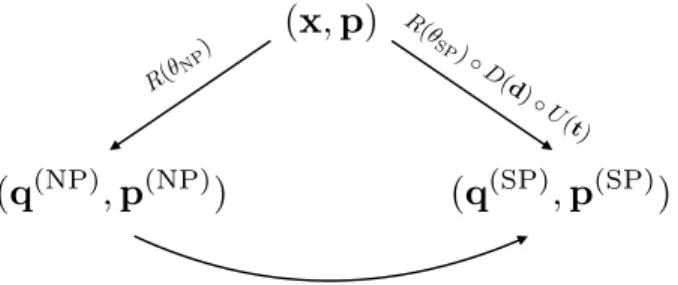
FIG. 1. Diagram of the coordinate transformations that di-agonalize the thermodynamic limit of the Dicke Hamiltonian both in the NP and SP. The original pair of canonical coor-dinates(x,p) in Eqs. (4, 5) are transformed via a rotation R(θNP) to diagonalize the Hamiltonian in the NP. For the

SP the transformation is more involved, requiring to com-pose a translation represented byU(t), a dilationD(d)and

another rotation R(θSP). The overall transformation that

links NP and SP coordinates is easily obtained by compos-ing successive transformations (see also Appendices B and C). The explicit parameters that enter in the transformations

are t = ( √

2Ω

ω

√

N(1−µ2)

ω ,−

√

N(1−µ)

∆ ), tan(2θSP) = 2ω∆µ2 µ2_ω2−∆2, tan(2θNP) =4Ω

√

ω∆

ω2−∆2 andd= (1, √

2µ

1+µ).

yields

HSP=ωc†c+∆(1+µ) 2µ d

†_d₊∆(1−µ)(3+µ) 8µ(1+µ) (d

†₊_d₎2 (3)

+Ωµ √

2 1+µ(c

†₊_c₎₍_d†₊_d_{) −}N 2 (

2Ω2

ω +

∆2ω

8Ω2),

whereµ= (ω∆)/(4Ω2) = (Ωc/Ω)2,α= (Ω/ω)√N(1−µ2₎ andβ=√N(1−µ)/2.

In the thermodynamic limit, HNP and HSP capture, separately in each phase, the thermodynamic properties of the Dicke model. More specifically, one can interpret them as an effective description of the dominating Gaus-sian fluctuations of the order parameter far from the crit-ical region. As such, this description is rather generic for many-body statistical systems undergoing a discrete symmetry breaking. As shown below, the specific choice of the Dicke model as an example allows us to more eas-ily establish the connection between the relevant fluctu-ations in the two phases.

Hereafter, we neglect the 1/N corrections inHNP/SP, which is equivalent to taking the thermodynamic limit

(3)

Since HNP and HSP are quadratic, they can be diagonalized via appropriate generalized Bogolyubov transformations42_{. However, for our purposes it is more} convenient to work in the aforementioned 2DHO sentation and consider the associated coordinate repre-sentationx= (x, y),p= (px, py):

x= √1

2ω(a+a

†₎_, _p x=i

√_ω

2(a

†₋_a₎_, ₍₄₎

y= √1

2∆(b+b †₎_, _p

y=i

√

∆ 2(b

†₋_b₎_, ₍₅₎

where [x, px] = [y, py] = i and all other commutators vanish. In each phase, the Bogolyubov transformation which diagonalizes HNP/SP becomes a geometric

trans-formation of the coordinates, namely a combination of rotationsR, dilationsD and translationsU as shown in Fig. 1. In their diagonal bases, the Hamiltonians are written in terms of new coordinates q(ν) = (_q(ν)

x , q(yν)), p(ν) = (_p(ν)

x , p(yν)) (ν = NP/SP) and have fundamental frequencies

ω(ν)

± =

¿ Á Á Á Á À1₂⎛⎜

⎝ω

2₊∆2

j2 ν

± ¿ Á Á

À(ω2₋∆2

j2 ν

)

2

+16jνΩ2ω∆

⎞ ⎟ ⎠

(6)

withjNP=1 andjSP=µ.

IV. LOSCHMIDT AMPLITUDE

A fundamental quantity which characterizes the work statistics is the Loschmidt amplitude13

L(t) = ⟨GS(Ω0)∣e−itHNP(Ω)∣GS(Ω0)⟩, (7) with ∣GS(Ω0)⟩ denoting one of the two superradiant ground states at maximal transverse magnetization, i.e. chosen as the ground state ofHSP(Ω0)+Jxfor→0+ (the other one would be obtained by minimizing the en-ergy for →0−_{, corresponding to} _Jx → −_Jx_{). Without}

loss of generality, we rescale the energies so that the NP ground state has zero energy.

Inserting four completeness relations in (7), the Loschmidt amplitude becomes

L(t) = ∫ d2q(SP)

1 d2q

(SP)

2 d2q

(NP)

1 d2q

(NP)

2 ⟨GS(Ω0)∣q(1SP)⟩ ×

× ⟨q(SP)

1 ∣q

(NP)

1 ⟩ ⟨q

(NP)

1 ∣e

−itHNP∣_q(NP)

2 ⟩ ×

× ⟨q(NP)

2 ∣q

(SP)

2 ⟩ ⟨q

(SP)

2 ∣GS(Ω0)⟩, (8) In the expression above, we note that: (i)⟨GS(Ω0)∣q

(SP)

1 ⟩ and ⟨q(SP)

2 ∣GS(Ω0)⟩ are the ground state wavefunc-tions of the SP two-dimensional harmonic oscillator and are therefore (as functions of q(SP)

1/2 ) Gaussians with

zero mean and variances (1/

√ ω(SP)

+ ,1/

√ ω(SP)

− ); (ii)

⟨q(NP)

1 ∣e

−itHNP∣_q(NP)

2 ⟩ is the propagator of the NP two-dimensional oscillator, and thus has a complex Gaus-sian structure which becomes purely GausGaus-sian after a Wick rotation to imaginary timet→ −is; (iii) the over-laps ⟨q(NP)

j ∣q

(SP)

j ⟩ correspond to a change of variable (see Appendices B and C) in the integration accord-ing to the canonical transformation mappaccord-ing q(NP) ↔

q(SP) _{(see Fig. 1), which can be expressed as} _q(SP) =

Sq(NP) +√_N_T_{, where we introduced the shorthand}

S=R(θSP)D(d)R−1(θNP)and

√

NT=R(θSP)D(d)tin relation to the sketch in Fig. 1. The problem of calculat-ingL(t)is now reduced to a Gaussian integration, which can be solved exactly to yield a large deviation form

L(t) =A(t)eN l(t)

, (9)

where both the function l(t) and the prefactor A(t)

are intensive functions, i.e. do not depend on N. To write them in a compact form, we introduce three diagonal matrices QSP = diag(ω

(SP)

+ , ω

(SP)

− ), P±(t) =

±idiag(ω(NP)

+ (tan(

ω(NP)+ t

2 ))

±1

, ω(NP)

− (tan(

ω−(NP)t

2 ))

±1

)

and

K±(t) =S ⊺

QSPS+P±(t). (10)

In terms of these matrices, the rate function reads

l(t) = −T⊺(

QSP−QSPSK+−1(t)S ⊺

QSP)T, (11) while the prefactor is

A(t) = ¿ Á Á Á

À −4 detD2ω

(NP)

+ ω

(NP)

− ω

(SP)

+ ω

(SP)

−

sin(ω(NP)

+ t)sin(ω

(NP)

− t)detK+(t)detK−(t)

.

(12)

V. STATISTICS OF WORK

The Loschmidt amplitude calculated above gives ac-cess to the statistics of the work done by the quench Ω0 → Ω, as shown in14. The average work per atom

w = WN/N is a stochastic variable with a distribution

P(w) whose generating function is the analytical con-tinuation of L(t) to imaginary time t → −is. In the large-N limit, L(−is) can be written as in Eq. (9) by substitution. The probability P(w) must therefore ful-fill a large deviation principle as well, namely P(w) ∝

exp(−N p(w)) and furthermore the rate function p(w)

and the SCGF l(−is) are related by a Legendre trans-form p(w) = −infs∈R(ws+l(−is)) (Gartner-Ellis

(4)

(c)

p

(

w

)

(b)

p

(

w

)

(a)

w

w s

s⇤ +

s⇤

wc= l0(s⇤) s⇤+

0.8 0.85 0.9 0.95 1.5

2 2.5 3

-2 0 2 4

0 1 2 3

Ê Ê Ê Ê Ê Ê ÊÊ ÊÊ Ê

Ê ÊÊ

ÊÊÊÊÊÊÊÊÊÊÊÊÊÊÊÊÊÊÊÊ ÊÊÊÊÊ

ÊÊÊÊ ÊÊÊ

ÊÊÊ ÊÊÊ

0 0.1 0.2 0.3 0.4 0.5 0.2

0.4 0.6

-2 0 2 4 6 8 10

-1 0 1 2

Ê Ê

Ê Ê Ê Ê ÊÊÊÊÊÊ ÊÊ

ÊÊ ÊÊ

ÊÊ Ê

Ê ÊÊ

Ê Ê

0 1 2 3 4

1 2 3 4 5

Ê Ê

Ê Ê Ê

ÊÊ ÊÊÊ

ÊÊÊ Ê ÊÊ Ê

Ê ÊÊ Ê

Ê ÊÊ Ê ÊÊ Ê Ê Ê Ê Ê Ê Ê Ê Ê Ê Ê Ê Ê Ê Ê Ê Ê Ê Ê Ê Ê Ê Ê Ê Ê

Ê

0 1 2 3 4

-2 -1 0 1 2 3

w

p

0(w

)

rate function

l

(

is

)

w

s

Legendre transform

l

(

is

)

scale cumulant generating function

µSP= ⌦2c/⌦20 µNP

=

⌦

2 /c

⌦

2

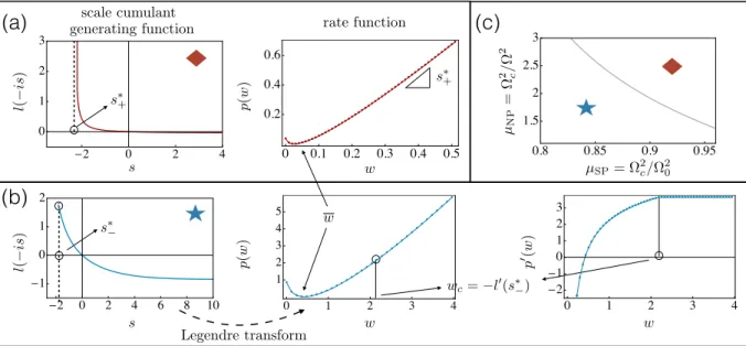
FIG. 2. Phase transitions in the work distributionp(w)obtained as the Legendre transform of the SCGFl(−is)Eq. (11) (at

fixedω=1). (a) The SCGFl(−is) diverges as s→s∗+. Correspondingly, p(w), which is obtained by a Legendre transform

(LT) froml(−is), approaches asymptotically the linear regime with slope−s∗+forw≫w(withwthe typical value of the work,

i.e. the one for whichp(w) =0). This scenario is the one expected for the models that belong to the class B introduced in

Ref.14. (b) The singular behavior ofl(−is)is controlled bys∗− which is approached at finite value with finite derivativel ′

(s∗−).

The LT thus displays a non-analytical point inwc= −l′(−is∗−)andp(w) = −s ∗

−w forw>wc. This non-analytical point of the

rate function corresponds to a phase transition in the rare fluctuations of the work. Plots in (a) and (b) are obtained with the same ∆=0.8 and Ω=0.3 by tuning the superradiant coupling from Ω0=0.47 to Ω0=0.9. (c) Analytical (diamond) and

non-analytical (star) domains ofp(w) in the planeµNP-µSP withµNP=Ω2c/Ω2 and µSP=Ω2c/Ω20 at ∆=0.8. At fixed Ω, the

non-analytical point appears only if the quench starts deep enough in the SP. The solid line denotes the boundary between the two areas and is where the non-analyticity inp(w)appears.

The 2DHO model has no upper bound to its energy spectrum and thus should belong to class B, according to Ref.14_{. However, in some parameter regimes its SCGF}

l(−is)reaches the leftmost point of its domain with fi-nite (instead of diverging) derivative, see Fig. 2(b). This property ofl(−is)translates in a non-analytical behavior ofp(w), which was not previoulsy reported.

The appearance of such a regime is directly related to the domain ofL(−is) = ⟨GS(Ω0)∣e−sHNP(Ω)∣GS(Ω0)⟩. In performing the analytic continuation of (9), we thereby have to stop at the first singularity encountered. First, we note that for s ≥ 0 L(−is) is always well-defined. Second, a singularity of L(−is) can be either associ-ated to a singularity of SCGF l(−is) or of the ampli-tude A(−is) (or both). Third, for l(−is) this can only occur when detK+(−is) =0, whereas forA(−is)

singular-ities can additionally emerge when detK−(−is) =0. We

denote by s∗

± the rightmost singular point of K±(−is).

We remark that sin(ω(NP)

+ t)sin(ω

(NP)

− t)detK−(t)

t→0

→ ω(NP)

− ω

(NP)

+ /4, curing the singularity in s = 0 and

im-plying s∗

−<0. The left domain edge of L(−is) is

there-fore max(s∗

+, s

∗

−). Two regimes can thus be identified:

if s∗

+ > s

∗

−, the SCGF l(−is) diverges at its leftmost

point (corresponding to class B of Ref.14). Correspond-ingly, p(w) approaches asymptotically a linear regime with slope −s∗

+ for w → +∞, as sketched in Fig. 2(a).

If insteads∗

+ <s

∗

−, then l(−is) remains finite and

differ-entiable ins∗

−, signalling a different qualitative behavior.

This in fact yields a point of non-analyticity inp(w) lo-cated atwc= −l′(−is∗−) < +∞, sketched in Fig. 2(b). For

all w> wc, p(w) = −s∗

−w−l(−is

∗

−) exactly,

correspond-ing to a jump in the second derivative of p(w), which vanishes for w > wc, see Fig. 2(b). The emergence of either scenario depends on the pre- and post-quench pa-rameters Ω0, Ω, ω and ∆. In Fig. 2(c) we provide an example showing the emergence of these two regions for ∆=0.8,ω=1 and various values of Ω0and Ω. These are produced by numerically solving detK+(−is) =0.

Finally, we remark that quenches within the NP have already been studied in29_{. In that case, log}_L₍_t₎_{is not} proportional to N (extensive) and therefore a large de-viation behavior does not emerge. The NP to SP and the SP to SP protocols will be investigated the object of future investigations.

VI. DISCUSSION AND CONCLUSIONS

(5)

statis-tics of the work exhibits in this regime a non-analytical point, signaling an out-of-equilibrium phase transition in the rare fluctuations of the work. It is important to stress that the physical intepretation of a non-analytical point in this context is not straightforward and deserves by itself a more detailed and quantitative investigation. Our current intuition is based on similar works in the context of classical stochastic44–46 _{(or more generally,} dissipative47–56_{) systems. There, non-equilibrium phase} transitions in the rare fluctuations of some observable (typically a current) are associated to a sharp change in the nature of the “typical” configurations the sys-tem displays when the observable (current) is biased to-wards values far from its average. Similarly, we think that the qualitative nature of quantum states populated when large fluctuations of the work are encountered may change sharply on the two sides of the transition, but further studies are required to establish whether this is the case.

It would be also interesting to understand what rela-tion there is between the non-analiticities found here and the dynamical phase transitions investigated in57.

Acknowledgements—The research leading to these re-sults has received funding from the European Research Council under the European Unions Seventh Framework Programme (FP/2007-2013)/ERC Grant Agreement No. 335266 (ESCQUMA). P.R. acknowledges funding by the European Union through the H2020 - MCIF No. 766442. I.L. gratefully acknowledges funding through the Royal Society Wolfson Research Merit Award. The authors wish to thank M. Heyl and A. Gambassi for useful dis-cussions at a preliminary stage of the project and H. Touchette for useful comments on the manuscript.

A. Dicke model and Holstein-Primakoff transformation

The exact form in the thermodynamic limit of the ground state of the Dicke model can be worked out both in the normal (NP) and in the superradiant phase (SP) through a suitable Holstein-Primakoff transforma-tion. Let us consider the Dicke Hamiltonian:

HD=ωa†a+∆Jz+ Ω

√

N(a+a

†₎_Jx_, ₍₁₃₎

where theJα_{’s (}_α₌_{x, y, z}_{) form an irreducible} represen-tation of the angular momentum of dimension N/2. In the large-N limit we can employ the following Holstein-Primakoff transformation:

Jz=b†b−N/2, J+=

b†√N−b†b , J−=√

N−b†b b ,

(14)

where b, b† satisfy ordinary bosonic commutation rela-tions. This leads to:

HD=ωa†a+∆b†b−

N∆

2 + (15)

+Ω(a+a†)⎛ ⎝b†

√

1−b†b

N +

√

1−b†b

N b ⎞ ⎠.

In the thermodynamic limit we can naively ignore the terms proportional to 1/√N. In this way we obtain a solvable quadratic bosonic model. This works in the NP at small Ω, but this approximation breaks down in the SP for Ω large enough, signaling that a quantum phase transition is taking place. In the following we analyze separately the two different phases obtaining the corre-sponding effective Hamiltonians. We will focus, in par-ticular, on the coordinate representation, that will be useful to evaluate the Loschmidt amplitudes. The re-sults summarized here in the following two subsections are extensively covered in21_.

B. Normal phase

In the NP we omit the 1/√N terms so that Eq. (15) reduces to

HNP=ωa†a+∆b†b+Ω(a+a†)(b+b†) −

N∆

2 . (16) This Hamiltonian can be diagonalized by a suitable Bo-goliubov transformation that mixes the four different cre-ation and annihilcre-ation operators. However the picture is simpler if we switch to the coordinate space, by writing:

x=√1

2ω(a+a

†₎_, _p x=i

√_ω

2(a

†₋_a₎_, ₍₁₇₎

y=√1

2∆(b+b †₎_, _p

y=i

√

∆ 2(b

†₋_b₎_. ₍₁₈₎

In this way, it is easy to realize that a rotation in the

(x, y)-plane puts the Hamiltonian in a diagonal form. In particular we need the following coordinate transforma-tion:

q(NP)= (

q(NP)

x , q

(NP)

y )

⊺=

R(θNP)x, (19)

R(θ) = (₋cos_sin(₍θ_θ)₎ sin_cos(₍θ_θ)_{) )} (20)

withθNPgiven by:

tan(2θNP) =

4Ω√ω∆

ω2₋_∆2 . (21)

The eigenfrequencies of the Hamiltonian in the NP read:

ω(NP)

± =

√

1 2(ω

(6)

It follows from Eq. (22) that the potential is not bounded from below for Ω > √ω∆/2 = Ωc, thus signaling that this effective Hamiltonian description breaks down at strong coupling. Before moving to the analysis of the SP, we notice that the ground state of the NP in the coordinate basisq(NP) _{is a 2-dimensional Gaussian}

cen-tered around q(NP) = (₀_,₀) _{with variance} (_σ

x, σy) =

(1/

√ ω(NP)

+ ,1/

√ ω(NP)

− ).

C. Superradiant phase

The derivation of the effective Hamiltonian in the SP is more involved. We refer to21 _{for the details. Here we} only report the fundamental results that we will need in the following to compute the Loschmidt amplitude cor-responding to the quench for the NP to the SP. Starting from Eq. (15) we define two new operatorsc=a−√α,

d=b+√β and we choose the displacement parameters properly in order to eliminate the terms linear in the bosonic operators. In this way we get an effective Hamil-tonian for the SP, that reads:

HSP=ωc†c+∆(1+µ) 2µ d

†_d₊∆(1−µ)(3+µ) 8µ(1+µ) (d

†₊_d₎2 (23)

+Ωµ √

2 1+µ(c

†₊_c₎₍_d†₊_d_{) +}_const_.

where µ = (ω∆)/(4Ω2_{) = (}_Ωc_/_Ω₎2_{. Again we focus on} the coordinate space representation. In order to get the diagonal form of the hamiltonian in the SP, we need to apply three succesive canonical transformations, firstly a translation represented by the vectort= (tx, ty)(which is the transformation that allows to getHSPfrom Eq. (15)), then a dilation D(d)on the y coordinate and finally a rotation by an angleθSP. In formulas:

q(SP)=

R(θSP)D(d)(x+t), (24) where the explicit parameters of the transformation are:

t=⎛

⎝ √

2Ω

ω √

N(1−µ2₎

ω ,

√

N(1−µ)

∆

⎞

⎠, (25)

tan(2θSP) = 2ω∆µ 2

µ2_ω2₋_∆2, (26)

d= (1,

√

2µ

1+µ). (27)

In the new coordinates of Eq. (24) the effective Hamil-tonianHSPis diagonal with eigenfrequencies given by:

ω(SP)

± =

¿ Á Á Á Á À1₂⎛⎜

⎝ω

2₊∆2

µ2 ±

¿ Á Á

À(ω2₋∆2

µ2) 2

+4ω2_∆2⎞_⎟

⎠.

(28)

Again, in the coordinate basisq(SP) _{the ground state of}

the SP is a Gaussian centered aroundq(SP)= (₀_,₀)_and

with variances(σx, σy) = (1/

√ ω(SP)

+ ,1/

√ ω(SP)

− ).

Finally, combining Eqs. (20) and (24), we obtain the explicit relation between NP and SP coordinates that we extensively use in the main text:

q(SP)=

Sq(NP)+√

NT, (29)

S=R(θSP)D(d)R(θNP)⊺, (30)

√

NT=R(θSP)D(d)t. (31)

D. Harmonic oscillator propagators and Gaussian integrals

We consider first a standard quantum harmonic oscil-lator Hamiltonian

HHO= p 2 2m+

m

2ω 2

q2. (32)

Its propagator, defined on the position basis as

F(q1, q2, t) = ⟨q1∣e−itHHO∣q2⟩, (33) connects any state∣ψ(t0)⟩at timet0with its time-evolved counterpart at timet0+tvia the relation

ψ(q1, t0+t) ≡ ⟨q1∣ψ(t0+t)⟩ = ∫

+∞

−∞

dq2F(q1, q2, t)ψ(q2, t0), (34) withψ(q, t) = ⟨q∣ψ(t)⟩ denoting the corresponding wave-function. The functional form of the propagator is known and reads

F(q1, q2, t) = (

mω

2πi̵hsin(ωt))

1 2

e2̵himωsin(ωt)[(q 2

1+q₂2)cos(ωt)−2q1q2]

.

(35) This formula can be straightforwardly generalized to any set ofnuncoupled harmonic oscillators by simply taking the product:

F(n)(

q1,q2, t) = ∏ i

Fi(q1,i, q2,i, t). (36)

In our case, it is sufficient to stop at two, whose coordi-nates we labelq = (qx, qy)⊺, whose masses are set to 1 and whose frequencies are denoted by(ω+, ω−). Working

in natural units (̵h=1) yields

F(2)(_q

1,q2, t) = 1 2πi(

ω+ω−

sin(ω+t)sin(ω−t)

) 1 2

×e2 sin(iωω++t)[(q 2

1,x+q2₂_,x)cos(ω+t)−2q1,xq2,x]

×

×e2 sin(iωω−−t)[(q 2

1,y+q2₂_,y)cos(ω−t)−2q1,yq2,y]

,

(37)

(7)

form of F is always that of a (complex) Gaussian func-tion, which can also be more compactly expressed as

F(2)(_q

1,q2, t) = 1 2πi(

ω+ω−

sin(ω+t)sin(ω−t)

) 1 2

e−1₂q⃗⊺_M

⃗

q

(38) with the shorthand q⃗⊺ = (

q⊺

1,q

⊺

2) = (q1,x, q1,y, q2,x, q2,y) and

M =1⊗Pd+σx⊗Pmix, (39)

where we defined

Pd= ( −iω+cot₀ (ω+t) ₋_iω 0

−cot(ω−t) )

(40)

and

Pmix= (iω+csc₀(ω+t) _iω 0

−csc(ω−t) )

. (41)

These expressions can be simplified by performing a rota-tion on the “1-2” components mappingσx_→_σz _{in (39),}

which transformsM into a block diagonal matrix

(P+ 0

0 P−

) (42)

withP±=Pd±Pmix defined as in the main text.

The ground state ∣GS⟩ of a harmonic oscillator also displays a Gaussian wavefunction and in our case it can be expressed as

⟨q∣GS⟩ = (ω+ω−

π2 )

1 4

e−ω₂+q_x2−ω₂−q2_y = (ω+ω−

π2 )

1 4

e−1₂q⊺Qq

(43) with

Q= (ω+ 0

0 ω−

). (44)

The expression of the Loschmidt amplitude is therefore a Gaussian integral which can be reduced to the form

G(A,b) = ∫ ddqe−1₂q⊺Aq−b⊺⋅q ₍₄₅₎

withAad×dan invertible, diagonalizable matrix whose eigenvalues have positive real part andbad-dimensional vector. This integral yields

G(A,b) = 1 (2π)d2

√

detAe

1 2b

⊺_A−1_b

. (46)

1

L. F. Cugliandolo, eprint arXiv:cond-mat/0210312 (2002), cond-mat/0210312.

2

A. Crisanti and F. Ritort, Journal of Physics A: Mathe-matical and General36, R181 (2003).

3

C. Jarzynski, Annual Review of Condensed Matter Physics 2, 329 (2011), https://doi.org/10.1146/annurev-conmatphys-062910-140506.

4

J. Berges, S. Bors´anyi, and C. Wetterich, Phys. Rev. Lett.

93, 142002 (2004).

5 _{A. Polkovnikov, K. Sengupta, A. Silva, and M.} Vengalat-tore, Rev. Mod. Phys.83, 863 (2011).

6

M. Rigol, V. Dunjko, V. Yurovsky, and M. Olshanii, Phys. Rev. Lett.98, 050405 (2007).

7

P. Calabrese, F. H. L. Essler, and M. Fagotti, Phys. Rev. Lett.106, 227203 (2011).

8

M. Greiner, O. Mandel, T. W. H¨ansch, and I. Bloch, Na-ture419, 51 (2002).

9

T. Kinoshita, T. Wenger, and D. S. Weiss, Nature440, 900 (2006).

10 _{M. Gring, M. Kuhnert, T. Langen, T. Kitagawa, B. Rauer,} M. Schreitl, L. Mazets, D. A. Smith, E. Demler, and J. Schmiedmayer, Science337, 1318 (2012).

11 _{M. Esposito, U. Harbola,} _{and S. Mukamel, Rev. Mod.} Phys.81, 1665 (2009).

12

M. Campisi, P. H¨anggi, and P. Talkner, Rev. Mod. Phys.

83, 771 (2011). 13

A. Silva, Phys. Rev. Lett.101, 120603 (2008). 14

A. Gambassi and A. Silva, Phys. Rev. Lett.109, 250602

(2012). 15

C. P. Espigares, P. L. Garrido, and P. I. Hurtado, Phys. Rev. E87, 032115 (2013).

16

N. Tiz´on-Escamilla, C. P´erez-Espigares, P. L. Garrido, and P. I. Hurtado, Phys. Rev. Lett.119, 090602 (2017). 17

R. Dicke, Phys. Rev.93, 99 (1954).

18 _{F. Dimer, B. Estienne, A. S. Parkins,} _{and H. J.} Carmichael, Phys. Rev. A75, 013804 (2007).

19

D. Nagy, G. K´onya, G. Szirmai, and P. Domokos, Phys. Rev. Lett.104, 130401 (2010).

20

K. Hepp and E. Lieb, Phys. Rev. A8, 2517 (1973). 21

C. Emary and T. Brandes, Phys. Rev. E67, 066203 (2003). 22

K. Baumann, C. Guerlin, F. Brenneke, and T. Esslinger, Nature (London)464, 1301 (2010).

23

K. Baumann, R. Mottl, F. Brennecke, and T. Esslinger, Phys. Rev. Lett.107, 140402 (2011).

24

J. Klinder, H. Keßler, M. Wolke, L. Mathey, and A. Hem-merich, PNAS112, 3290 (2015).

25

S. Gammelmark and K. Mølmer, New J. Phys.12, 053035 (2011).

26

L. Bakemeier, A. Alvermann, and H. Fehske, Phys. Rev. A85, 043821 (2012).

27 _{O. Casta˜}_{nos, E. Nahmad-Achar, R. L´}_opez-Pe˜_{na, and J. G.} Hirsch, Phys. Rev. A86, 023814 (2012).

28

M. J. Bhaseen, J. Mayoh, B. D. Simons, and J. Keeling, Phys. Rev. A85, 013817 (2012).

29

(8)

30

P. Strack and S. Sachdev, Phys. Rev. Lett. 107, 277202 (2011).

31

M. Buchhold, P. Strack, S. Sachdev, and S. Diehl, Phys. Rev. A87, 063622 (2013).

32 _{P. Rotondo, E. Tesio, and S. Caracciolo, Phys. Rev. B}₉₁_, 014415 (2015).

33

S. Gopalakrishnan, B. Lev, and P. Goldbart, Phys. Rev. Lett.107, 277201 (2011).

34

P. Rotondo, M. Cosentino Lagomarsino, and G. Viola, Phys. Rev. Lett.114, 143601 (2015).

35

P. Domokos and H. Ritsch, Phys. Rev. Lett. 89, 253003 (2002).

36

S. Zippilli, G. Morigi, and H. Ritsch, Phys. Rev. Lett.93, 123002 (2004).

37 _{J. K. Asb´}_{oth, P. Domokos, H. Ritsch, and A. Vukics, Phys.} Rev. A72, 053417 (2005).

38

A. T. Black, H. W. Chan, and V. Vuleti´c, Phys. Rev. Lett.

91, 203001 (2003). 39

K. Hepp and E. Lieb, Ann. Phys.76, 360 (1973). 40

Y. K. Wang and F. T. Hioe, Phys. Rev. A7, 831 (1973). 41

See Supplementary Material. 42

N. Bogolyubov, J. Phys. (USSR)11, 23 (1947). 43

H. Touchette, Physics Reports478, 1 (2009). 44

T. Bodineau and B. Derrida, Phys. Rev. E 72, 066110 (2005).

45

N. Tiz´on-Escamilla, C. P´erez-Espigares, P. L. Garrido, and P. I. Hurtado, Phys. Rev. Lett.119, 090602 (2017). 46

P. I. Hurtado and P. L. Garrido, Phys. Rev. Lett. 107, 180601 (2011).

47 _{S. Genway, J. M. Hickey, J. P. Garrahan,} _{and A. D.} Armour, ArXiv e-prints (2012), arXiv:1212.5200 [cond-mat.stat-mech].

48

J. M. Hickey, S. Genway, I. Lesanovsky, and J. P. Garra-han, Phys. Rev. B87, 184303 (2013).

49

J. M. Hickey, S. Genway, and J. P. Garrahan, Phys. Rev. B89, 054301 (2014).

50

J. M. Hickey, ArXiv e-prints (2014), arXiv:1403.5515 [cond-mat.stat-mech].

51

E. Aghion, D. A. Kessler, and E. Barkai, Phys. Rev. Lett.

118, 260601 (2017). 52

M. ˇZnidariˇc, Phys. Rev. Lett.112, 040602 (2014). 53

D. Manzano and P. I. Hurtado, Phys. Rev. B 90, 125138 (2014).

54

F. Carollo, J. P. Garrahan, I. Lesanovsky, and C. P´ erez-Espigares, Phys. Rev. E96, 052118 (2017).

55

A. Kundu, S. Sabhapandit, and A. Dhar, Journal of Sta-tistical Mechanics: Theory and Experiment2011, P03007 (2011).

56

S. Sabhapandit, Phys. Rev. E85, 021108 (2012). 57

M. Heyl, A. Polkovnikov, and S. Kehrein, Phys. Rev. Lett.