High precision lateral distortion measurement and correction in coherence scanning interferometry using an arbitrary surface

High-precision lateral distortion measurement

and correction in coherence scanning

interferometry using an arbitrary surface

P

1_{Industrial Metrology and Optics, Production Engineering, KTH Royal Institute of Technology, SE-100}

44 Stockholm, Sweden

2_{Manufacturing Metrology Team, Faculty of Engineering, The University of Nottingham, Nottingham}

NG7 2RD, UK

*_{[email protected]}

Abstract: Lateral optical distortion is present in most optical imaging systems. In coherence scanning interferometry, distortion may cause field-dependent systematic errors in the measurement of surface topography. These errors become critical when high-precision surfaces, e.g. precision optics, are measured. Current calibration and correction methods for distortion require some form of calibration artefact that has a smooth local surface and a grid of high-precision manufactured features. Moreover, to ensure high accuracy and precision of the absolute and relative locations of the features of these artefacts, requires their positions to be determined using a traceable measuring instrument, e.g. a metrological atomic force microscope. Thus, the manufacturing and calibration processes for calibration artefacts are often expensive and complex. In this paper, we demonstrate for the first time the calibration and correction of optical distortion in a coherence scanning interferometer system by using an arbitrary surface that contains some deviations from flat and has some features (possibly just contamination), such that feature detection is possible. By using image processing and a self-calibration technique, a precision of a few nanometres is achieved for the distortion correction. An inexpensive metal surface, e.g. the surface of a coin, or a scratched and defected mirror, which can be easily found in a laboratory or workshop, may be used. The cost of the distortion correction with nanometre level precision is reduced to almost zero if the absolute scale is not required. Although an absolute scale is still needed to make the calibration traceable, the problem of obtaining the traceability is simplified as only a traceable measure of the distance between two arbitrary points is needed. Thus, the total cost of transferring the traceability may also be reduced significantly using the proposed method. Published by The Optical Society under the terms of the Creative Commons Attribution 4.0 License. Further distribution of this work must maintain attribution to the author(s) and the published article’s title, journal citation, and DOI.

OCIS codes: (100.0100) Image processing; (100.5010) Pattern recognition; (110.0110) Imaging systems; (120.3940) Metrology; (150.1488) Calibration; (180.0180) Microscopy.

References and links

1. M. Born and E. Wolf, Principles of Optics: Electromagnetic Theory of Propagation, Interference and Diffraction of Light, 7th ed. (Cambridge University Press, 1999), Chap. 5.

2. A. Henning, C. Giusca, A. Forbes, I. Smith, R. Leach, J. Coupland, and R. Mandal, “Correction for lateral distortion in coherence scanning interferometry,” Ann. CIRP 62(1), 547–550 (2013).

3. P. Ekberg and L. Mattsson, “A new 2D self-calibration method with large freedom and high-precision performance for imaging metrology devices,” in Proceedings of the 15th International Conference of the European Society for Precision Engineering and Nanotechnology (Elsevier, 2015), pp. 159–160.

4. S. Yoneyama, H. Kikuta, A. Kitagawa, and K. Kitamura, “Lens distortion correction for digital image correlation by measuring rigid body displacement,” Opt. Eng. 45(2), 023602 (2006).

5. P. de Groot, “Principles of interference microscopy for the measurement of surface topography,” Adv. Opt. Photonics 7(1), 1–65 (2015).

6. P. de Groot, Optical Measurement of Surface Topography, R. K. Leach, ed. (Springer, 2011), Chap. 9.

7. R. Leach, C. Giusca, D. Cox, M. Guttmann, P.-J. Jakobs, and P. Rubert, “Development of low-cost material measures for calibration of the metrological characteristics of surface topography instruments,” Ann. CIRP 64(1), 545–548 (2014).

8. J. Haycocks and K. Jackson, “Traceable calibration of transfer standards for scanning probe microscopy,” Precis. Eng. 29(2), 168–175 (2005).

9. R. K. Leach, C. L. Giusca, and K. Naoi, “Development and characterization of a new instrument for the traceable measurement of areal surface texture,” Meas. Sci. Technol. 20(12), 125102 (2009).

10. P. Ekberg, L. Stiblert, and L. Mattsson, “A new general approach for solving the self-calibration problem on large area 2D ultra-precision coordinate measurement machines,” Meas. Sci. Technol. 25(5), 055001 (2014). 11. C. L. Giusca, R. K. Leach, F. Helary, T. Gutauskas, and L. Nimishakavi, “Calibration of the scales of areal

surface topography-measuring instruments: part 1. Measurement noise and residual flatness,” Meas. Sci. Technol. 23(3), 035008 (2012).

12. M. Sutton, J. Orteu, and H. Schreier, Image Correlation for Shape, Motion and Deformation Measurements: Basic Concepts, Theory and Applications, (Springer, 2009).

13. C. Evans, R. Hocken, and W. Estler, “Self-calibration: reversal, redundancy, error separation, and ‘absolute testing’,” Ann. CIRP 45(2), 617–634 (1996).

14. M. Raugh, “Absolute two-dimensional sub-micron metrology for electron beam lithography – a calibration theory with applications,” Precis. Eng. 7(1), 1–13 (1985).

1. Introduction

Lateral optical distortion is present in most optical imaging systems. Distortion, unlike optical aberrations such as spherical aberration, coma and astigmatism, is not responsible for a lack of sharpness of the image; rather it is related to the form of the image, and the degree of the distortion is dependent on the position in the image plane [1]. Optical aberrations are usually suppressed for optimisation of the optical resolution in a commercial coherence scanning interferometry (CSI) system, but a significant amount of distortion can be present [2,3].

In areas such as computer vision, distortion in a camera system may cause errors in pattern analysis and recognition, dimensional and displacement measurement, three-dimensional (3D) image reconstruction, etc [4]. In a 3D imaging system that measures the surface topography and geometry of an object, distortion may cause errors in the dimensional measurement in both lateral and height directions. For example, in CSI [5,6], distortion may cause field-dependent systematic errors in the measurement of surface topography. Thus, distortion should be corrected in order to achieve a non-distorted image field and a uniform lateral sampling distance of the image projected on to the camera, such that the measurement accuracy can be improved.

The correction of lateral distortion in an imaging system can be divided into two steps: 1) correct the form of the image, e.g. when imaging a perfect grid pattern the systematic deformation of this grid should be removed so that the measured grid has uniformly distributed nodes; 2) absolute calibration and adjustment of the scale, i.e. measurement of the distance between any two points within the image should be made traceable to the definition of metre, which is a linear scaling problem.

The traditional calibration and adjustment of the lateral distortion for a 3D imaging system combines the two steps listed above into one by measuring a standard artefact. The artefact usually contains a grid of precision manufactured patterns, mostly with rectangular or circular shapes, e.g. an areal cross grating standard [7]. The distortion is then calculated as the deviation of the measured positions of the patterns compared to their nominal positions. The nominal positions are calibrated by a traceable metrological instrument, e.g. a metrological atomic force microscopy (AFM) [8] or stylus instrument [9]. The manufacturing and calibration processes of the standard artefact are often complex and expensive.

The major disadvantages of the traditional correction and current self-calibration methods are their strong dependence on structured grid patterns. Problems include: 1) the accuracy of the locations of the patterns limits the accuracy of the distortion correction if traditional methods are used; 2) the tolerance on the manufacturing quality of the surface topography (form and texture) is very tight; 3) the edges of the pattern structures need to be sharp and clean, and the uncertainty of the necessary edge detection algorithm degrades the accuracy of the distortion correction; 4) care must be taken when handling and storing the artefacts in order to ensure low levels of damage or contamination; and 5) availability – for correction of different imaging systems with different lenses and magnifications, a range of grids with suitable pitches is required.

In this paper, a new methodology for the correction of lateral distortion in a CSI system, based on a simple sub-pixel image correlation method and self-calibration, will be demonstrated. Instead of using a manufactured grid pattern, an arbitrary surface is used and a precision of a few nanometres is achieved for the distortion correction. Here, an arbitrary surface refers to a surface that contains some deviations from flat and has some features (possibly just contamination), such that feature detection is possible. This surface could be a rough surface, e.g. a regular machined metal surface or the surface of a coin, or it could be a smooth surface with random features or structured patterns, e.g. a scratched and defected mirror or an (uncalibrated) areal cross grating. These surfaces can be easily found in a laboratory, manufacturing workshop and even an office. The method demonstrated in this paper may significantly enhance the precision of the distortion correction of 3D optical imaging systems. The cost of the artefact may be reduced significantly and even to zero if the absolute scale is not considered.

2. Methods

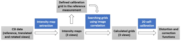
The distortion correction method contains three parts – image generation, image processing and self-calibration. The correction process is illustrated in Fig. 1. In the first step of the process, the intensity images of different measurements are extracted from the 3D CSI data of the surface. Usually three measurements are needed for self-calibration [10]. In this paper, the first measurement is called reference measurement based on which a calibration grid will be defined, the second one being the translated measurement with translation approximately one pitch of the grid and the third one being the rotated measurement with approximately 90° rotation. Second, all the three measurements are repeated five times for evaluating measurement overlay which is the limiting factor of the precision of the self-calibration result. The defined calibration grid is searched in the repeated reference measurements and each translated and rotated measurement by using a sub-pixel image correlation method. In principle, the grids calculated from the repeated reference measurements should overlay the defined grid, and the grids calculated from the translated and rotated measurements should appear distorted. In the last step, the averaged reference, translated and rotated measurements will be input to the self-calibration algorithm, and the outcome is the distortion and correction functions.

2.1 Extractio

CSI is an int emitting diod using a broad modulates the from a surfac impulse resp comparing th reference sur measured. Th interference s The detailed p

When per acquired by s axial interfere (DC) term an separated in t intensity sign filter. The int distance but distortion cor estimate the b a CSI system compensated dimensional ( further analys

Fig. 2 interfe freque

The CSI maximum sca nm and is ca lenses used in

on of intensity

erferometric im de (LED) that u dband source is

e interference ce is concentra ponse with os he complex am rface and the hus, the height

signal. In the la principles of C

rforming an a scanning the C ence signal (se nd an oscillat the spatial freq nal without the tensity value ( is not as sens rrection result, best focus posit m should mat

for optimisati (2D) intensity sis.

2. Extraction of 2 erence signal reco ency part correspo

instrument us an speed of 96 alculated using n this study are

y map from 3D

maging techniq usually operate s that the shape signal such th ated in a smal scillating term mplitude of th

light wave re variation is en ateral direction SI can be foun areal surface CSI imaging sy ee Fig. 2(a) an ting modulatio quency domain

e interference (DC term) of sitive as the fr the areal heig tion along the ch the cohere on of the accu map. The inte

2D intensity map orded by a pixel; c onds to the intensity

sed in this st 6 μm/s. The su g the averaging

given in Table

D CSI data

que that uses es in the visib e of the source

at the power o ll distance in m (i.e. fringes he light wave eflected or ba ncoded into the n, CSI works v nd elsewhere [5

topography m ystem axially.

nd Fig. 2(b)). on term. Thes

(see Fig. 2(c) effect, can be each pixel ma fringes. For ac ght information axial direction ence envelope uracy and robu ensity map, as

in CSI. a) Interf c) the Fourier tran y map; d) the extra

tudy has a pr rface topograp g method [11] e 1.

a broadband s ble spectrum. T e spectrum (usu of the interfero the axial direc s). The interf e reflected fro ack-scattered fr e phase and coh very similarly t

5,6].

measurement, Each pixel of

The signal co se two terms ). The DC term e extracted by

ay also vary w chieving a hig n obtained from n for each pixel e. Any offset,

ustness of the shown in Fig

ferometirc image nsform of the sign

acted intensity ma

recision piezo phy repeatabili ]. The specific

source, such a The major adv ually close to G ometric signal ction, in analo ference is rea om a flat and from the surfa herence envelo to ordinary mic

a series of im f the camera re

ontains a direc of the signal m, correspondi using a low-p with the axial gh precision an m the fringes i

l. Note that the if present, sh extraction of g. 2(d), will be

stack in CSI; b) nal, where the low ap.

o-electric drive ity is approxim cations of the

s a light-antage of Gaussian) response ogy to an alised by d smooth ace to be ope of the

croscopy.

mages is ecords an ct current l may be ing to the pass (LP) scanning nd robust is used to e focus of hould be f the two-e ustwo-ed for

) w

e with a mately 0.1

Table 1. Specifications of the objective lenses

Magnification 50 × (1 × zoom) 5.5 × (1 × zoom)

Interferometer type Mirau Michelson

NA 0.55 0.15

Optical resolution /μm 0.52 1.90

Field of view (FOV) /mm 0.167 1.507

Spatial sampling /μm 0.163 1.472

2.2 Sub-pixel image correlation method

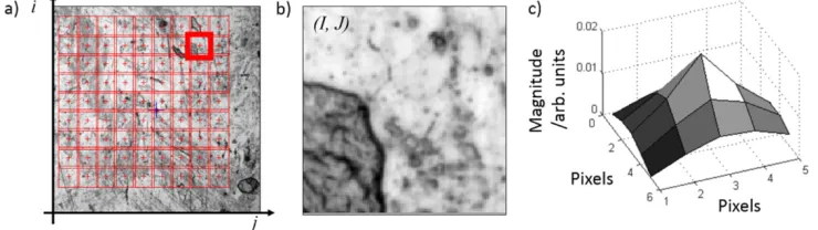
Image correlation methods have been widely applied in many areas, such as the measurement of stress, strain and displacement in the field of mechanics [12]. In this study, the first step of the image correlation method is the definition of the calibration grid of image patches in the 2D intensity map extracted from the measured CSI data of a surface (see Fig. 3). The same area of the surface that covers the defined grid is also measured in the translated and rotated views. The defined grid in the image of an arbitrary surface is equivalent to the physical calibration grid manufactured in a standard artefact. One of the advantages is that the location and pitch of the defined grid is known and may be easily adjusted so that any spatial frequency of the distortion can be captured.

Fig. 3. Illustration of the image correlation method. a) 9-by-9 grid of image patches defined in the 2D intensity map of the CSI measurement of a coin surface; b) the enlarged image patch (100-by-100 pixels) of which the centroid is located at (I, J) in the image coordinate; c) the correlation function, which is the result of searching for the reference image patch around (I, J) in the translated or rotated views.

Searching for the exact positions of the image patches (e.g. see Fig. 3(b)) in the translated and rotated measurements is based on the calculation of the cross-correlation function between two image patches; one from the reference measurement and the other from the translated or rotated measurement. This process does not require high precision and is carried out by using a priori information of the translation and rotation, i.e. the nominal translated distance and the degree of the rotation angle. The cross-correlation function can be expressed as

( )

(

) (

)

, , , , ,

I J

j i

C p q =



respectively. Functions f(i, j) and g(i, j) are the intensity maps of the image patches in the reference view and the translated or rotated view, respectively. Because the images of all three views are aligned using a priori knowledge of the translation and rotation, the searching area can be as small as a few pixels around (I, J). The pixel coordinates (p, q), corresponding to the correlation maximum, are the desired quantities. The entire set of (p, q) for all image patches provides the location of the defined grid with pixel-precision in the translated or rotated view.

The result of the correlation function is refined with sub-pixel precision, which can be achieved by resampling the image patches using a cubic interpolation combined with a simple iterative method for searching for the correlation maxima.

2.3 The 2D self-calibration method

Reversal techniques and other forms of self-calibration have been used for centuries in order to calibrate machine tools and measuring instruments [13]. The mathematical theory behind the 2D self-calibration technique in metrology systems was developed by Raugh [14]. A numerical approach for solving the self-calibration problem, based around the concept of iteration, was developed by Ekberg et. al. [10]. In general, 2D self-calibration is based on the assumption that the artefact will not change its shape regardless of how it is mounted in the measuring instrument, i.e. it is a rigid body. Then the apparent shape of the artefact will change when it is observed at different positions in the measuring instrument, if lateral distortion is present. It is possible to separate the distortion and the real shape of the artefact, by using at least three measurements of the same artefact with different placements. The typical placement scheme contains a reference measurement, a translated measurement and a measurement with the artefact rotated 90°. The details of the 2D self-calibration method can be found elsewhere [3,10].

In the 2D self-calibration method, measurement overlay limits the precision of the result. In an optical imaging system, overlay is a quantity that evaluates how well the system repeats the measurement result in the lateral directions, i.e. the relative positions of features in the repeated images of a surface should not change. The absolute positions of features in the images may change due to some systematic shift of the entire image domain. Ideally, the overlay value should be of the same magnitude as the measurement noise.

3. Results

3.1 Image generation and processing result

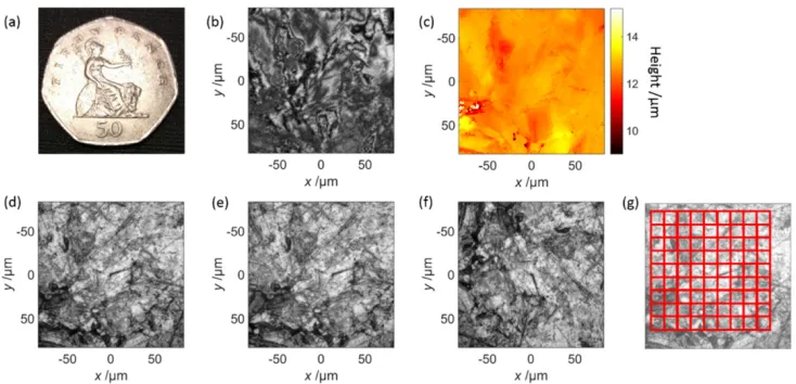
Fig. 4. Extraction of the 2D intensity maps from CSI measurements of a coin surface and definition of the grid. a) Photograph of the coin; b) an image slice from the 3D fringe data; c) calculated height map; d, e, f) Intensity maps of the reference, translated and rotated views, respectively; g) defined grid and image patches. The grey scales of all intensity images are normalised. The 50 × objective lens was used.

The nominal grid is defined as a perfect square area containing 9-by-9 image patches as shown in Fig. 4(g). The centroids of the image patches are calculated using the described image correlation method, such that the grid can be presented by 9-by-9 nodes. Figure 5 shows the grids that are calculated from the five repeated measurements of the three different views. As shown in Figs. 5(a)-5(c), the measured grids from the translated and rotated views are distorted because of the presence of optical distortion.

It is noted that the repeated measurements are not overlapping perfectly, which indicates possible lateral drifts of the image domains of the repeated measurements. The drift can be evaluated as the relative offsets of the centroids of the grids (see Fig. 5(d)-5(f)). The drift is of the order of tens of nanometres and is probably caused by the motion of the axial scanner or the stage. The drift of the entire image domain can hardly be noticed in a scanning-type microscopic imaging system, where the lateral sampling distance in an image is usually in the range from 100 nm to 6 µm. The drift may degrade the repeatability of the instrument.

Fig. 5. Measured grids from three different views. a, b, c) Resulting grids (absolute coordinates) of the repeated measurements of the reference, translated and rotated views, respectively (the errors are magnified for visualisation purpose); d, e, f) calculated drifts for the reference, translated and rotated views, respectively. The 50 × objective lens was used.

The image processing result of the same CSI system using 5.5 × magnification lens (with the FOV of 1.5 mm) is shown in Fig. 6. The calculated drift and overlay are of the same magnitude compared to those of 50 × lens, which provides evidence that the overlay and drift are determined by the system but not the image processing algorithm. The overlay is mainly determined by the measurement noise and the drift is caused by some systematic motion in the system.

3.2 Self-calibration result

The input to the self-calibration algorithm is the measured grids from the three different views, as shown in Fig. 7(a) (aligned with the centroids for display purposes). The output is the distortion map (Fig. 7(b)), from which the distortion function and the correction function can be obtained [2]. By applying the correction function to the three measurements, the distortions in the translated and rotated views can be corrected (see Fig. 7(c)). Due to the system noise, the distortion cannot be completely compensated. The overall quality of the self-calibration result is evaluated by the residual errors after the distortion correction, and the evaluation is carried out by calculating the root-mean-square (RMS) value of the residual errors for the three views. The result is given in Table 2. The RMS residual error is approximately 2 nm.

Fig. 7. Self-calibration result. a) Input to the self-calibration algorithm and the placement scheme; b) calculated distortion of the CSI system with 50 × objective lens; c) overlay of the distortion-corrected grids.

Table 2. Distortion correction result for the 50 × objective lens

Distortion /nm RMS residual error /nm

Maximum Reference view Translated view Rotated view

x 72 1.6 1.5 2.2

y 50 1.7 1.4 2

Fig. 8. Self-calibration result. a) Input to the self-calibration algorithm and the placement scheme; b) calculated distortion of the CSI system with 5.5 × objective lens; c) overlay of the distortion-corrected grids.

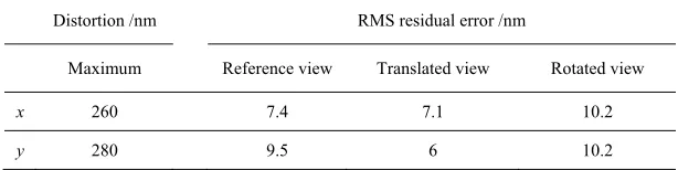
Table 3. Distortion correction result for the 5.5 × objective lens

Distortion /nm RMS residual error /nm

Maximum Reference view Translated view Rotated view

x 260 7.4 7.1 10.2

y 280 9.5 6 10.2

4. Conclusion

The method demonstrated in this paper provides a new methodology for lateral distortion correction in 3D optical imaging systems. Unlike the traditional method, in which the distortion correction has to rely on some precision-manufactured and calibrated standard artefact with structured patterns, the new approach makes use of an arbitrary surface that can be easily found, e.g. a coin surface, such that the spatial sampling of the distortion is no longer limited by the structures in the artefact. A precision of a few nanometres can be achieved for the distortion correction over a large FOV. A rarely observed drift, of the order of a few tens of nanometres, due to the motion of the axial scanner or the translation stage in the measuring system has also been found. Although an absolute scale is still needed to make the calibration traceable, the problem of obtaining the traceability is simplified as only an accurate measure of the distance between two arbitrary points is needed. Thus, the total cost of transferring the traceability may be reduced significantly using the new approach. In the future, a new method that may simplify the way of obtaining the absolute scale will be investigated, and a 2.5D self-calibration method will be developed for correction of field curvature effects in CSI.

Funding

Engineering and Physical Sciences Research Council (grant number EP/M008983/1); European Metrology Programme for Innovation and Research([grant number 15SIB01). Acknowledgements