Measuring nonlinear signal combination using EEG

Measuring nonlinear signal combination using EEG

Darren G. M. Cunningham

Nottingham Visual Neuroscience, School of Psychology, University Park Campus, University of Nottingham,

Nottingham, Nottinghamshire, UK

$

Daniel H. Baker

#

$

Jonathan W. Peirce

Nottingham Visual Neuroscience, School of Psychology, University Park Campus, University of Nottingham,

Nottingham, Nottinghamshire, UK

#

$

Relatively little is known about the processes, both linear and nonlinear, by which signals are combined beyond V1. By presenting two stimulus components simultaneously, flickering at different temporal frequencies (frequency tagging) while measuring steady-state visual evoked potentials, we can assess responses to the individual components, including direct measurements of suppression on each other, and various nonlinear

responses to their combination found at intermodulation frequencies. The result is a rather rich dataset of

frequencies at which responses can be found. We

presented pairs of sinusoidal gratings at different temporal frequencies, forming plaid patterns that were‘‘coherent’’

(looking like a checkerboard) and‘‘noncoherent’’(looking like a pair of transparently overlaid gratings), and found clear intermodulation responses to compound stimuli, indicating nonlinear summation. This might have been attributed to cross-orientation suppression except that the pattern of intermodulation responses differed for coherent and noncoherent patterns, whereas the effects of

suppression (measured at the component frequencies) did not. A two-stage model of nonlinear summation involving conjunction detection with a logical AND gate described the data well, capturing the difference between coherent and noncoherent plaids over a wide array of possible response frequencies. Multistimulus frequency-tagged EEG in combination with computational modeling may be a very valuable tool in studying the conjunction of these signals. In the current study the results suggest a second-order mechanism responding selectively to coherent plaid patterns.

Introduction

Relatively little is known about how the visual system encodes representations beyond oriented bars and edges

in V1 (for a review, see Peirce, 2015). We do know that the visual system is nonlinear in various ways. It uses suppressive nonlinear operations to normalize response properties (e.g., Carandini & Heeger, 2012), which might serve to reduce redundancy in the neural representation of natural scenes (e.g., Schwartz & Simoncelli, 2001). Nonlinear processes are also necessary to perform logical AND operations driving selective responses to particular stimulus combinations (Gheorghiu & King-dom, 2009; Peirce, 2007a, 2011). These might be useful in detecting various features such as a curved contour (the AND operation of at least two neurons with abutting receptive fields and slightly different orienta-tions: Gheorghiu & Kingdom, 2009; Hancock & Peirce, 2008) or coherent plaid (the AND operation of two neurons with spatially overlapping receptive fields but different tuning).

The existence of multiple nonlinearities in response to compound stimuli poses the methodological prob-lem of having to disentangle them for individual examination. Psychophysical approaches and func-tional magnetic resonance imaging (fMRI) measure the summed nonlinear response to stimuli, making them unsuitable for this particular task. Electroencephalog-raphy (EEG) responses, however, may be more applicable. Responses to sensory stimuli can be measured by frequency tagginga stimulus, temporally modulating its intensity at a fixed rate and measuring the entrained neural response at the same temporal frequency. Multiple stimuli can be tagged simulta-neously by using a different temporal frequency for each stimulus (for a review, see Norcia, Appelbaum, Ales, Cottereau, & Rossion, 2015; Regan, 1983 Regan & Heron, 1969; Regan & Regam, 1988; Spekreijse & Reits, 1982; Zemon & Ratliff, 1984). We can, for

example, present stimuli at 5 and 7 Hz, allowing us to measure independently the response to each stimulus at 5 Hz (f1) and 7 Hz (f2), and thus examine the effect of one stimulus on the response to another by masking, for example.

Furthermore, intermodulation responses at the difference (f2f1: 2 Hz) and sum (f1þf2: 12 Hz) of these fundamental frequencies can also be measured. These, and their harmonics, indicate a nonlinearity at or after the point of summation (for a mathematical explanation, see Regan & Regan,1988) although, on their own, intermodulation responses do not tell us what mechanism may have caused them (e.g., a suppressive mechanism or an AND gate).

Several recent studies have employed measurements of responses at intermodulation frequencies to examine signal combinations in visual cortex. Boremanse, Nor-cia, and Rossion (2013) presented half-face stimuli at two different frequencies and measured the sum and difference intermodulation responses. These were larger when two face halves were presented as a whole face compared to when they were separated vertically or horizontally. They attribute this to a nonlinear mecha-nism sensitive to the whole, rather than the parts, of the face. Similarly, intermodulation responses have been found when parts of a Kanizsa-type illusory stimulus (Kanizsa, 1979) are presented at different rates (Alp, Kogo, Van Belle, Wagemans, & Rossion, 2016; Gund-lach & M¨uller, 2013), when a texture is distinct from its background in a figure–ground experiment (Appelbaum, Wade, Pettet, Vildavski, & Norcia, 2008) and when the abutting sides of a square are moved closer together during perceptual form-motion binding (Aissani, Cot-tereau, Dumas, Paradis, & Lorenceau, 2011).

Intermodulation responses have also been used to study normalization processes using grating and plaid stimuli. Tsai, Wade, and Norcia (2012) found that the sum intermodulation term amplitude peaked when a test pattern was masked by a pattern of equivalent contrast but disappeared when contrasts were different. Also, Candy, Skoczenski, and Norcia (2001) and Baker, Norcia, and Candy (2011) presented pairs of oriented gratings at different temporal frequencies and found intermodulation responses when they were parallel in orientation. In both cases, intermodulation responses can be explained as suppressive interactions between units.

The nonlinearity giving rise to the intermodulation response beyond these early normalization processes may also involve an additional nonlinear mechanism sensitive to the compound stimulus of two gratings, an AND gate responding to plaids. Particular combina-tions of gratings form the ‘‘coherent’’ percept of a distinct checkerboard pattern, while other ‘‘noncoher-ent’’ combinations appear more readily as two semi-transparent, superimposed gratings (Adelson & Movshon,1982; Meese & Freeman, 1995). Contrast

adaptation has been found to plaids above and beyond that expected by adaptation to the components (Mc-Govern & Peirce, 2007; Peirce & Taylor, 2006;

Robinson & MacLeod, 2011), but only when the spatial frequency of the components was matched (Hancock, McGovern, & Peirce, 2010). Similarly, a visual search task has suggested pre-attentive mechanisms sensitive only to coherent plaid patterns (Nam, Solomon, Morgan, Wright, & Chubb, 2009).

This dependence on coherence for the putative plaid detector presents a possible way to distinguish the nonlinearities feeding the intermodulation response. If special mechanisms for plaids exist and are partially driving the intermodulation responses, then we would expect such intermodulation responses to differ ac-cording to the coherence. Conversely if the intermod-ulation response is driven by a normalization pool for cross-orientation suppression (XOS), which is thought to be relatively untuned to spatial frequency (De-Angelis, Freeman, & Ohzawa,1994; Petrov, Carandini, & McKee, 2005), then the intermodulation response should be similar for different forms of plaid.

Here, we compare intermodulation responses to a range of grating combinations, including both coherent and noncoherent plaid patterns. To create noncoherent patterns we used substantially different spatial fre-quencies (1 and 3 cpd for the two components) that have previously been found to result in clear nonco-herent patterns in moving stimuli (Adelson & Mov-shon, 1982). If the intermodulation responses are caused only by suppressive mechanisms, we would expect to find it in both forms of compound pattern. Conversely, if the intermodulation response results both from suppressive mechanisms and mechanisms sensitive to plaid patterns then we would expect to find larger intermodulation responses to coherent plaids but similar levels of component suppression for both coherent and noncoherent plaids. We generated a multilayer network model with XOS in Layer 1 and a combinatorial AND gate in Layer 2 and found that it described the data well.

Methods

Participants

Apparatus and materials

A computer-controlled LCD monitor (Iiyama Prolite X2472HD, Iiyama, Hoofddorp, The Nether-lands) with a screen resolution of 192031080 pixels, mean luminance of 133.17 cd/m2, and a refresh rate of 60 Hz was used for stimulus presentation. The gamma function of the screen was linearized using a pho-tometer (ColorCal MKII, Cambridge Research Sys-tems, Kent, UK). Participants sat at a screen distance

of approximately 100120 cm, depending on how they

felt comfortable; this was measured for each partici-pant and used to maintain a constant stimulus size measured in degrees of visual angle. The PsychoPy stimulus generation library (Peirce,2007b) was used for stimulus presentation and collecting participant responses to a simple detection task. A button box (Cedrus RB-830 Response Pad, Cedrus Corporation, San Pedro, CA) was used for participants to make these responses.

EEG data acquisition

A DBPA-1 Sensorium bio-amplifier (Sensorium Inc., Charlotte, VT) was used for EEG recording at a sampling rate of 1000 Hz. Voltage responses were recorded from 122 electrode channels (silver/silver-chloride) on a set of customized whole-head caps with twisted and fixed electrode cables (EasyCap, Munich, Germany). This included a ground electrode placed on the forehead, reference electrode at the left mastoid, EOG electrodes (RHE, LHE, and LIO), and 117 scalp electrodes. Caps were centered on electrode Cz, halfway between the nasion and inion. Where possible, impedances were brought below 25 kilohms (kX) before the experiment began (below 50 kXif this could not be achieved). Note that on many commercial systems this might seem like high impedance, but is the suggested setting for the Sensorium DBPA-1 amplifier.

A parallel port from the stimulus computer was used to indicate when a stimulus onset occurred, sending a trigger signal time-locked to the screen refresh. We confirmed in advance that this was precise on our hardware, using a photometer connected to the amplifier via a StimTracker (Cedrus Light Sensor, Cedrus Corporation).

Stimuli and experimental procedure

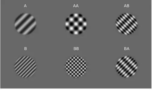
Stimuli comprised of two sinusoidal gratings (de-noted as ‘‘A’’ and ‘‘B’’) and various combinations thereof. Grating A had a spatial frequency of 1 cpd and Grating B a spatial frequency of 3 cpd. These could then be combined with a second, spatially orthogonal

grating to form plaid patterns that were either coherent (‘‘AA,’’ ‘‘BB’’) or noncoherent (‘‘AB,’’ ‘‘BA’’) as shown in Figure 1. On each trial the overall orientation of the stimulus, either grating or plaid, was randomly

assigned, but the orthogonal configuration of the grating components that formed a plaid was main-tained.

Components were presented within a 7.58-diameter circular window with a raised cosine edge profile (width ¼1.58). In the center of the stimulus a further circle (diameter 0.48) was placed with the same midgray color as in the background, also with a raised cosine edge profile (0.088). This was done to accentuate the fixation dot, a red circle subtending 0.1758 in the center of the screen. A further green dot (0.258 diameter) appeared occasionally and briefly, located at a radius of 3.758

from the centrally located fixation point but a random radial angle. This was used as part of the attentional control task that participants were asked to perform. When seated in the recording booth, participants were instructed to maintain fixation on the central red fixation point. They had to conduct an attentional task independent of the stimulus presentation to ensure that attention was constant, a practice common in fMRI studies since the finding that differential attention to different stimuli can provide an important confound (Huk, Ress, & Heeger,2001). In our attentional control task participants were instructed to respond as quickly as possible when they detected the appearance of the green task dot (without looking towards it) by pressing the central button on the response box. This green dot appeared at a random time within any trial number

divisible by 10 or 6 (6, 10, 12, 18, etc.). This resulted in rare events, unpredictable to the participants, that required their attention to detect, preventing them from assigning greater or lesser attention to the actual stimulus. Although diverting attention away from the stimulus might decrease our chances of measuring strong signals (Appelbaum et al., 2009) we considered it more important to keep attention constant. It remains very possible, however, that we underestimate the size of responses in our data as a result of this. The percentage of task occurrences across each condition relative to the grand total number of occurrences shows no bias towards any particular condition (A1: 13.33%; A2: 13.07%; B1: 14.67%; B2: 10.67%; A1A2: 12.27%; B1B2: 13.33%; A1B2: 9.60%; B1A2: 13.07%). It is therefore unlikely that the dot task was a factor in determining any systematic effects observed between conditions. Participants responded to 76.34% (SEM¼

2.22) of dot occurrences, indicating that the task was neither too easy nor too difficult.

A brief presentation of the experiment was provided to ensure the participants understood what they were being asked to do. Following this, they were presented with a blank fixation screen consisting of a gray background and red fixation dot until they indicated that they were ready to begin.

To generate the intermodulation responses in plaid conditions, the two grating components had to have their contrast intensity simultaneously modulated at slightly different temporal frequencies. The frequencies chosen to do so were 2.3 and 3.75 Hz on the basis that they allowed the response frequencies to be temporally incommensurate; the fundamental frequencies (2.3, 3.75 Hz), their harmonics (2f1: 4.6 Hz, 2f2: 7.5 Hz) and the intermodulation terms (f2f1: 1.45 Hz,f1þf2: 6.05 Hz) and harmonics (2f22f1: 2.9 Hz, 2f1þ2f2: 12.1 Hz) would not overlap. Further, we aimed to avoid overlap between the typical alpha band (8–12 Hz) and the sum intermodulation response frequency (f1þ f2: 6.05 Hz) as in Boremanse et al. (2013) to boost signal to noise.

The contrast of any one component varied sinusoi-dally in time between 0%and 50% of the maximal contrast of the monitor (which had a maximal Michelson contrast of 0.99). The plaid patterns were formed from the signed sum (black is negative, white is positive) of the pixel values resulting from the two components such that, when the components were both at the peak of their sinusoidal modulation in time, a standard plaid pattern was physically present momen-tarily, whereas when either component was at its trough only the other component was physically present, as a simple grating. Due, presumably, to the reasonably high rate of contrast modulation the percept for the observer is not of two gratings changing contrast gradually. Rather the percept is still of a

pattern that alternates with gratings at a high and unpredictable rate. Movie 1 shows what a coherent plaid condition (A1A2) looked like.

For the remainder of this article, ‘‘1’’ denotes when a grating component was flickered at 2.3 Hz and ‘‘2’’ when flickered at 3.75 Hz. For example, Grating A flickered at 2.3 Hz will now be referred to as A1, while a coherent plaid with Grating A components will be referred to as A1A2, where one component was flickered at 2.3 Hz and the other at 3.75 Hz. This resulted in eight stimuli: four grating components (A1, A2, B1, and B2), two coherent plaids (A1A2 and B1B2), and two noncoherent plaids (A1B2 and B1A2). A trial consisted of an 11-s presentation of a flickering grating or two simultaneously flickering, superimposed grating components, followed by a 7–9-s interstimulus interval. Each of the eight stimuli was presented three times in a run, with five runs in total. Participants were given short breaks between runs. Upon completion, participants were thanked, debriefed, and given the opportunity to ask any questions.

Analytical procedure

Data were band-pass filtered between 0.1 and 100 Hz. They were then epoched according to stimulus onset, with the first second of data removed to exclude onset transients from the analysis, resulting in a 10-s epoch for each trial. Trials were time averaged by condition for each participant, averaging out activity that is not phase-locked to the stimulus presentation, such as the alpha-wave response. Fast Fourier trans-forms (FFTs) were then conducted on these average waveforms to bring the data into frequency space, resulting in amplitude responses (lV) at discrete frequencies (for a 10-s stimulus the FFT has a resolution of 0.1 Hz) between 0.1 and 100 Hz.

The amplitude response at each frequency at each electrode site was converted into a measure of signal-to-noise ratio (SNR) by dividing the amplitude at the frequency of interest by the average amplitude of the surrounding 12 frequency bins. The data used in the following analyses were taken from electrode Oz. This was based on group topographies showing peak responses for all stimuli occurring there, and is

consistent with measurements in the vicinity of primary visual cortex. We also conducted the analysis using a cluster of electrodes around Oz, but this made no difference to the conclusions from the analyses.

Initially, the frequencies of interest for analysis were atf1 (2.3 Hz), f2 (3.75 Hz),f2f1 (1.45 Hz), andf1þ f2 (6.05 Hz). Upon inspection of the data, responses at the 2f22f1 (2.9 Hz) and 2f1þ2f2 (12.1 Hz)

noise (SNR¼1), a series of one-sample t tests were conducted separately for each set of component SNRs (i.e., A1, A1A2, and A1B2; A2, A1A2, and B1A2; B1, B1B2, and B1A2; B2, B1B2, and A1B2), difference intermodulation SNRs (atf2f1 and 2f22f1: A1, A2, B2, A1A2, and A1B2), and sum intermodulation SNRs (atf1þf2 and 2f1þ2f2: A1, A2, B2, A1A2, and A1B2). Each series oft tests were corrected using the ranked Bonferroni-Holm method to control for Type 1 errors (Holm, 1979).

The extent to which grating/plaid pattern predicted response SNRs was examined using linear mixed-effects modeling. The analytical model was generated using the mixed function of the Afex package in R (Singmann et al.,2016). Grating/plaid pattern was the only predictor with random slopes as a function of ‘‘participant’’ using a maximal random effects structure (as recommended by Barr et al., 2013). This model was applied to both component SNRs and intermodulation SNRs. The lsmeans function in R for examining

pairwise comparisons from linear mixed-effects model structures was used when a significant main effect of pattern was found, and comparisons were corrected using the Tukey honest significance difference method for multiple comparisons (Russell, 2016).

Modeling

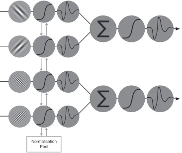
A two-layer network model was generated based on Peirce (2007a, 2011; see Figure 2) in which static sigmoidal nonlinearities were applied to the outputs of each channel (as expected by any model of V1 outputs) and simply summed by a ‘‘Layer 2’’ mechanism, which also has a sigmoidal nonlinearity. Such a model can be used to investigate the relationship between XOS, nonlinear additive summation, and the generation of intermodulation responses to plaids. Contrast input to the model was generated in the same way that contrast was modulated in the stimuli presented to participants:

contr¼C ðsinðtf2pÞ 0:5þ0:5Þ;

wheretrepresents a point in time between 0 and 11 s (in steps of 0.01 s),f the temporal frequency for that

component, andCthe maximum Michelson contrast

(set to 0.5). The multiplication and addition by 0.5 scaled the minimum and maximum contrast to be 0 and 1 initially and the further multiplication byCreduced the maximum contrast to 0.5.

Layer 1 involved four channels with static non-linearities (Naka & Rushton,1966) with an extra term in their denominators to account for XOS (Carandini & Heeger, 2012) and is here assumed to represent grating component responses. The structure of a Layer 1 channel was as follows:

compResp¼rMax I

n at

C50þIn atþNP

;

whererMaxis the maximum response of the channel,

Iat the input contrast of the stimulus component being

encoded at that channel at time pointt,nan exponent, andC50the semisaturation point. NP, used as the

normalization pool, is the sum of three extra terms corresponding to the input to the other three Layer 1 channels. The value of each of these terms was determined in a similar fashion to theIat term:

NP¼X

i¼3 In_it

The rMaxwas held constant at 1,n at 2, andC50at 0.2. Two channels corresponded to ‘‘detectors’’ for components A1 and A2, and their output was summed (CSa) before being passed to Layer 2. The same was

done for the other two channels, (B1 and B’) and their sum referred to as CSb.

The second layer can be thought of as two additional ‘‘channels’’ with a similar static nonlinearity (without the additional XOS term on the denominator), which would respond selectively to the presence of a plaid:

plaidResp¼rMax CS

n t

C50þCSnt

;

whereCS(either a or b) represents the linearly summed component responses (as described above), n an exponent, andC50the semisaturation point (the same used in Layer 1). As for the Layer 1 channels, rMax was held constant at 1, n at 2, andC50at 0.2. The overall output of the model was then calculated as the linearly summed response of compResp andplaidResp, simulating the population response measured with EEG.

It has been suggested that the temporal processing of signals by the mechanisms generating intermodulation responses may be key to their almost-always asym-metric response patterns (e.g., Alp et al., 2016; Boremanse et al., 2013). Thus, we wanted to evaluate the importance of neural impulse response functions (NIRs) on the performance of the model. Further, it has been suggested that later mechanisms in the visual pathway may differ in their temporal filtering proper-ties compared to earlier mechanisms. We therefore conducted simulations where NIRs were generated and used as temporal filters on each channel’s output.

We tested two variants of filter (Figure 3). The first variant was generated by summing three Gaussian distributions. It had a bandpass Fourier response peaking at ;5 Hz with a slow decay towards 20 Hz. The second form of linear filter was generated simply by halving the peaks and widths of the band-pass filter described above, resulting in a high(er)-pass Fourier response peaking at ;10 Hz. These filters were

combined in three ways: (a) the bandpass filter for both Layer 1 and Layer 2, (b) the bandpass filter for Layer 1 and higher frequency filter for Layer 2, and (c) no temporal filtering at either level. This allowed us to assess the importance of the temporal integration functions in the resulting responses, and whether there is any evidence for these differing in early- and late-stages of the model.

Following this, noise was added to the output of the model. A vector of values randomly sampled from a normal distribution (N¼10,000) was filtered with a third order bandpass Butterworth filter between 0.1 and 100 Hz. This resulted in a 1/f decay like that observed in the EEG data. The mean of the random distribution allowed us to scale the overall magnitude of the 1/fnoise and theSDthe degree of randomization

(M¼10 andSD¼0.5 for no NIR,M¼190 andSD¼

9.5 for application of NIR).

FFTs were performed on the model output with the added noise. The magnitude of model responses was normalized between 0 and 1 by using the minimum and maximum response for the condition being simulated. This controlled for the arbitrary scaling of model responses introduced by the temporal filter. In all cases, this maximum was found at the 1/f noise magnitude at 0.1 Hz, rather than at a signal bin related to the stimulus input. The same approach that was used for the EEG data was used to calculate SNRs at each frequency, and these were then used to perform model fitting.

Results

General overview

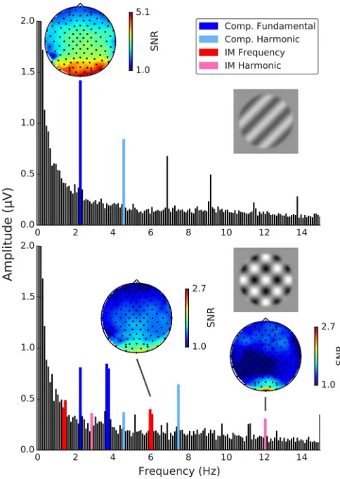
We wanted to measure fundamental responses to grating components, both alone and when forming part of a plaid. We also wanted to measure intermodulation responses at the difference and sum of the fundamental frequencies used to modulate the contrast of each component forming a plaid. Clear component-based responses atf1 (2.3 Hz) andf2 (3.75 Hz) were observed at posterior occipital sites for gratings presented alone as well as when they were presented along with another grating component in the plaid conditions. Further, clear intermodulation responses were observed in all plaid conditions atf1þf2 (6.05 Hz), but only in coherent plaid conditions at 2f1þ2f2 (12.1 Hz). In both cases these were observed at the same sites as the component responses (Figure 4).

Response to components

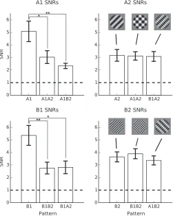
To test the well-documented effects of XOS (De-Angelis et al., 1994; Meese & Holmes, 2007; Petrov et al., 2005) we could compare directly the response to each frequency-tagged grating component in isolation and in the presence of a second grating. The SNR measures of these responses to each component— calculated by dividing the amplitude at the frequency of interest by the average amplitude of the surrounding 12 frequencies (with signal bins excluded)—can be seen in Figure 5. Substantial suppression was observed for components presented at 2.3 Hz in the presence of another grating component at 3.75 Hz. This was not the case for components presented at 3.75 Hz.

All fundamental component responses, whether presented alone or in the presence of another grating, were significantly above background noise (p,0.01 in all cases). For the 2.3 Hz response to grating A1 there was a significant main effect of stimulus pattern,F(2,

28)¼8.26,p¼0.002. Post hoc pairwise comparisons showed that component A1 SNRs were reduced for both the A1A2 plaid, t(28)¼2.92,p¼0.018, and the A1B2 plaid, t(28)¼3.91,p¼0.002, but there was no significant difference between the two plaid conditions, t(28)¼0.99,p¼0.587. A similar effect was observed for 2.3 Hz responses to B1,F(2, 28)¼6.64,p¼0.004, again driven by significant differences between the grating alone and each plaid condition (B1B2:t[28]¼3.12,p¼ 0.009; B1A2: t[28]¼3.12, p¼0.011). There was no significant difference between the response to coherent and noncoherent plaids, t(28)¼ 0.06,p¼0.998.

Figure 4. Example Fourier amplitude spectra with SNR topographies. Top: Grating component A1 alone with funda-mental SNR topography. Bottom: Coherent plaid A1A2 withf1þ

For the higher temporal frequency components, at 3.75 Hz the levels of suppression were less pronounced and did not result in significant main effects of stimulus type (A2:F[2, 28]¼0.02,p¼0.98; B2:F[2, 28]¼0.65,p ¼0.528). This pattern of suppression may reflect an

additional complex interaction between spatial and temporal frequency tuning of cross-orientation nor-malization processes (Cass & Alais,2006; Meese & Holmes, 2007, 2010).

In summary, although different patterns of sup-pression were observed between components, levels of XOS were similar for both coherent and noncoherent plaids for all conditions. This indicates that suppressive effects were not spatial-frequency tuned.

Response to plaids

Intermodulation frequencies were used to assess responses to the conjunction of grating components.

Responses at the difference frequency (f2f1: 1.45 Hz) were not prominent compared to background noise for all conditions. A main effect of pattern was found,F(6, 84)¼3.09,p¼0.009, though no significant differences were observed in post hoc pairwise comparisons between plaid conditions. At the harmonic of the intermodulation difference frequency (2f22f1: 2.9 Hz), responses in all conditions were not prominent compared to background noise, and the main effect of stimulus pattern on SNRs was nonsignificant, F(6, 84) ¼2.07,p¼0.066.

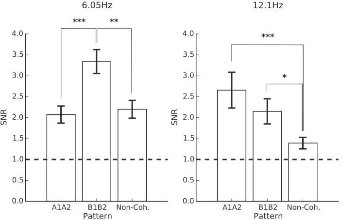
At the sum intermodulation frequency (f1þf2: 6.05 Hz) prominent responses were observed (Figure 6). One-samplet tests comparing each condition’s SNR to background noise revealed significant differences for both coherent plaid and noncoherent plaid conditions, A1A2: t(14)¼5.07,p¼0.001, 95% CI¼[1.62, 2.53]; B1B2: t(14)¼7.91,p ,0.001, 95%CI¼[2.70, 3.97]; A1B2: t(14)¼4.45,p¼0.003, 95%CI¼[1.66, 2.88]; B1A2: t(14)¼3.38, p,0.023, 95%CI¼[1.41, 2.84], as well as for component A2,t(14)¼3.24,p,0.024, 95%

CI¼[1.13, 1.65]. The latter finding was unexpected as only one component (i.e., only one flickering stimulus) was presented in that condition; mathematically, an intermodulation response should not take place. This finding is therefore likely spurious. A significant main effect of stimulus pattern was found,F(6, 84)¼24.23,p , 0.001. Post hoc pairwise comparisons showed that response SNRs at 6.05 Hz were significantly larger in response to plaid B1B2 than for plaid A1A2, t(84)¼ 4.22,p,0.001, and the mean 6.05 Hz response SNR to the noncoherent plaids (the mean of A1B2 and B1A2 responses; t[84]¼ 3.00,p¼0.009).

At the harmonic of the intermodulation sum frequency (2f1þ2f2: 12.1 Hz; see Figure 6) only responses to coherent plaids were significantly above background noise, A1A2: t(14)¼3.74,p¼0.017, 95%

CI¼[1.71, 3.60]; B1B2:t(14)¼4.00,p¼0.017, 95%CI

¼[1.48, 2.82]. There was a significant main effect of stimulus pattern on response SNRs,F(6, 84)¼11.61,p , 0.001. Significant differences were observed in post hoc pairwise comparisons between both coherent plaids and the mean noncoherent plaid response, A1A2: t(84)

¼4.69,p ,0.001; B1B2: t(84)¼2.62,p¼0.030.

In summary, responses at the difference intermodu-lation terms analyzed here were not significantly above background noise and did not systematically differ based on plaid coherence. The response at 6.05 Hz was significantly above background noise for all plaid conditions, and was greater for coherent plaid B1B2 than any other condition. That all plaid responses were significantly above background noise and that sup-pression for coherent and noncoherent plaid responses was similar, may indicate that the 6.05 Hz response primarily reflected XOS. A more convincing selectivity was observed at 12.1 Hz; it was larger for coherent than

noncoherent plaids, and was significantly above back-ground noise for coherent plaids but not for nonco-herent plaids, suggesting that it was spatial-frequency tuned.

Modeling

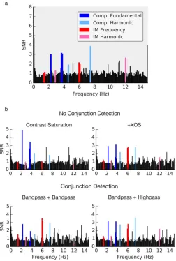
Simulations of several candidate models, including the conjunction detection model outlined in the Methodssection, were generated. The candidate models with no conjunction detection were each composed of a channel bank of four V1 neurons (like Layer 1 of the conjunction model). In the interest of understanding how different component-based non-linearities contribute to the summed nonnon-linearities observed in EEG data, input signals underwent only contrast saturation in one model, and both contrast saturation and XOS in another. The output of these simulations is shown in the top rows of Figures 7b and 8b. In both figures, the model output is being compared to the EEG data we collected for coherent plaid A1A2. The EEG data is shown in section (a) of both figures, and the various model outputs are shown in section (b). The same noise as described earlier was injected into the output of these. Two versions of each were run; one where no NIR was applied to the channel output (Figure 7b) and another where the NIRs that were outlined earlier were applied (Figure 8b). It should be noted that the application of the second NIR (whether bandpass or high pass) was applied to Layer 2 in the

conjunction detection model only (shown in the bottom row of Figures 7b and 8b).

In the first candidate model, each channel had a stage of contrast saturation upon contrast input (Figure 7b top left; Figure 8b top left). Fundamental responses and their harmonics were produced. No intermodulation responses were produced because the operation performed by each channel was independent of the other channels; the different temporal signals could not combine. This is dissimilar to the observed EEG data in sections (a) of both figures, and clearly not the case for much of the visual system. In V1

substantial XOS is usually observed in response to superimposed grating stimuli (e.g., Bonds, 1989; Brouwer & Heeger, 2011; Burr & Morrone, 1987).

The second candidate model performed contrast saturation and received input from a normalization pool (outlined in Methodssection)—that is, a model of contrast gain to account for contrast saturation and XOS (Figure 7b top right; Figure 8b top right). When no NIR was applied, suppression was observed at both the fundamental and harmonic component-based SNRs. With the application of the NIR to the output of each channel, suppression was observed at the funda-mental response frequencies, but the harmonic SNRs showed a slight increase. In both cases, a substantial intermodulation response SNR was observed at 6.05 Hz (f1þf2) and a slight intermodulation response was observed at 12.1 Hz (2f1þ2f1). This supports the finding that XOS drives substantial intermodulation responses (e.g., Baker et al., 2011; Candy et al., 2001). However, the output produced by these models is still

dissimilar to the raw data in showing relatively weak harmonic component responses (and essentially no harmonicintermodulationresponse).

When no NIR was applied, the additional nonline-arity of the conjunction detector raised the SNR at the fundamental, harmonic, and intermodulation terms compared to the contrast gain (contrast saturationþ XOS) only model. In contrast, the addition of the bandpass NIR at Layer 1 and the high-pass NIR at Layer 2 resulted in larger SNRs only at the harmonic responses (4.6 Hz: 2f1, 7.5 Hz: 2f2, and 12.1 Hz: 2f1þ 2f2). Applying the bandpass NIR to both Layers 1 and 2 of the conjunction model decreased fundamental component responses, the 4.6 Hz response and the 12.1

Hz response, but notably increased the 6.05 Hz response. This latter model was the most dissimilar of the conjunction detector models to the observed EEG data. The model with no NIR and the bandpassþ high-pass model both resulted in larger 12.1 Hz SNRs, the frequency at which a significant difference between coherent and noncoherent plaids was found in the EEG data. They also display several additional frequency combination responses that are present within the EEG data spectra, such as the response at 9.8 Hz (f1þ2f2). Both clearly capture some of the subtleties involved in the signal combinations taking place in the EEG data, though the larger 12.1 Hz response produced by the

Figure 7. SNR Spectra for (a) EEG data and (b) model data without an NIR being applied. Highlighted in dark blue are fundamental component-based SNRs (f1 andf2: 2.3 Hz and 3.75 Hz), light blue the component harmonic SNRs (2f1 and 2f2: 4.6 Hz and 7.5 Hz), red the intermodulation responses (f2f1 andf1þf2: 1.45 Hz and 6.05 Hz), and magenta the

intermodulation harmonic responses (2f22f1 and 2f1þ2f2: 2.9 Hz and 12.1 Hz). The contrast saturation model was the simplest, followed by the inclusion of XOS (normalization pool) and then the conjunction detection model.

bandpassþhigh-pass model is closer to the EEG findings.

In summary, we generated several simple fixed models to account for different kinds of signal summation in response to frequency-tagged flickering stimuli. Rather than comparing models using measures of fit quality and (somewhat arbitrary) penalties for numbers of parameters, we have compared models in terms of whether they produced responses at the expected frequencies. The only model variants capable of producing the full range of responses observed in the data were the models including a second layer

nonlinear step; the model with only XOS (normaliza-tion) does not show the observed intermodulation responses. The use of a bandpass NIR at Layer 1 and a higher pass NIR at Layer 2 of the conjunction model appears to slightly better account for our data than without the application of any NIR, and much better than when a bandpass NIR is applied to both Layers 1 and 2 of the model. This presumably indicates different temporal integration windows at different stages of the visual hierarchy.

Discussion

We have measured neural responses to sinusoidal grating patterns presented alone and combined as coherent and noncoherent plaids to assess the nonlinear combination of neural responses to the gratings. To do this we measured EEG responses at intermodulation frequencies, which have previously been shown to indicate a nonlinearity at or after the point of summation (Regan,1983; Regan & Heron, 1969; Regan & Regan, 1988; Spekreijse & Oosting, 1970; Spekreijse & Reits, 1982; Zemon & Ratliff, 1984). Our main finding was that for compound stimuli (plaids) we found reliable responses at 12.1 Hz (2f1þ2f2), but only when the combination formed a coherent plaid.

Although this intermodulation response indicates a nonlinear combination of signals, it does not tell us the nature of that nonlinearity. In particular it might simply reflect lateral suppressive effects such as XOS (Baker et al.,2011; Candy et al., 2001). The frequency-tagging technique we have used allows us to investigate that hypothesis directly by examining the effect of each component (e.g., presented at 3.75 Hz) on the response to the other (at 2.3 Hz). We did indeed observe substantial suppression; for example, when a compo-nent (either A1 or B1) was presented alone at 2.3 Hz, a greater 2.3 Hz response was observed than when the component was presented in combination with an orthogonal grating.

Critically, however, the 12.1 Hz response was very much dependent on the spatial frequencies being

matched in the two components. Conversely, and in keeping with previous findings that XOS is largely untuned for spatial frequency (DeAngelis et al., 1994; Petrov et al., 2005), the reductions in component responses that we measured occurred equally for any combination of spatial frequencies. It seems unlikely that the observed intermodulation responses resulted purely from XOS, given that one is tuned for spatial frequency and the other is not.

The perception of moving plaids has been shown to depend on matched spatial frequencies in several ways. When spatial frequencies differ in the two gratings being combined, observers perceive a pair of semi-transparent gratings sliding past each other (Adelson & Movshon,1982) whereas a plaid with matched spatial frequency components appears as a single coherent checkerboard pattern with a single direction of motion. Similarly, selective adaptation to static plaids decreases when components are unmatched (Hancock et al., 2010) and the pop-out effect in visual search disappears when plaid targets have unmatched components (Nam et al., 2009). A mechanism selective for coherent plaids appears to explain better the nonlinear intermodulation responses we have measured. In support of this, we found that the addition of ‘‘conjunction detector’’ channels beyond contrast gain operations resulted in model output more like the EEG data. A logical AND operation in combination with XOS cannot be ruled out as a candidate mechanism for driving plaid-selective responses at intermodulation frequencies.

Studies of fMRI (McDonald, Mannion, & Clifford,

2012) and positron emission topography (PET) (Wen-deroth, Watson, Egan, Tochon-Danguy, & O’Keefe, 1999) have shown similar responses to plaid and grating stimuli of equivalent contrast. McDonald et al. (2012) used fMRI to study the summation of signals to gratings and plaids. However, this method measures a mixed signal; it cannot distinguish changes in the responses of a set of neurons from changes in the number of neurons responding. For instance, a greater response in V1 could be caused either by reduced suppression between neurons or by recruitment of an additional mechanism. The inherently superior tempo-ral resolution of EEG, combined with the frequency-tagging technique, allows us to separate responses to different components within the stimulus.

Hz) and 2f2 (7.5 Hz)—not shown here—displayed the same effects as the fundamental responses in terms of component suppression; all components displayed the same amount of harmonic component suppression irrespective of plaid coherence.

The intermodulation responses we measured were predominantly observed at the sum intermodulation frequencies, and not at the difference. This has also been the case for several other intermodulation studies (Aissani et al.,2011; Alp et al., 2016; Appelbaum et al., 2008; Gundlach & M¨uller, 2013) but the converse was true for Boremanse et al. (2013). One interpretation for differences between the intermodulation terms sug-gested by Boremanse et al. (2013) is that responses at both frequencies reflect parallel nonlinearities but the sum intermodulation response output may be a temporally band- or high-pass nonlinearity and signal early local spatial interactions, whereas the difference intermodulation response may be generated by a temporally low-pass nonlinearity and generated by signal integration to higher level (global) stimuli, such as their face-part stimuli, which require longer to process (Alonso-Prieto, Van Belle, Liu-Shuang, Norcia, & Rossion, 2013). Here we found that the application of a bandpass temporal filter at Layer 1 and a higher frequency filter at Layer 2 of our model resulted in better model output than by applying a bandpass filter at both layers. Rapid local combinations would certainly fit in with our EEG results as we used simple sinusoidal gratings that presumably were being com-bined across many receptive fields to encode another pattern (the plaid). Further, sum intermodulation responses were strongest aroundOz, placed approxi-mately over the occipital pole, consistent with activity relatively early in visual cortex.

Alp et al. (2016) suggested that the temporal resonance properties of different neural mechanisms may influence the varied response at the difference and sum intermodulation frequencies. These resonances may depend on specific synaptic connections to and from the mechanisms, feedback connectivity and the relative complexity of the receptive field within the visual hierarchy (e.g., sensitive to compound plaids or sensitive to faces). The effects of such differences in temporal integration have not been applied quantita-tively in a computational model (e.g., to explain differential responses at sum- and difference-inter-modulation terms). Here we used a simple approach to model the temporal properties of mechanisms and found that using different neural impulse response functions (temporal filters) at early and late layers was sufficient to explain a wide range of features in the data. In the case studied here (plaid combinations) it

appeared that responses at 6.05 Hz (f1þf2) in the present data primarily represented XOS mechanisms,

while responses at 12.1 Hz (2f1þ2f2) reflected plaid-selective mechanisms.

The responses to gratings and plaids appear similar in terms of their topography. Although they may result from different neurons, we would expect these to be anatomically proximal. For example, if the response to plaids originated in V2, it would be hard to distinguish from the V1 response to gratings using EEG. Fur-thermore, although they are reliable, the intermodula-tion responses do not have large amplitudes, which compounds the difficulty in localizing them.

Conclusion

In summary, we have shown a nonlinear response to a compound of gratings (plaid) that does not arise purely from contrast normalization between spatial frequency channels. The data are in keeping with a mechanism for detecting conjunctions of visual fea-tures, as might result from a logical AND operation. The frequency-tagging technique provides a useful tool to investigate AND gates in a wide variety of neural mechanisms.

Keywords: plaids, gratings, EEG, midlevel, nonlinearity, intermodulation, frequency tagging

Acknowledgments

DC was funded by a studentship from the EPSRC, UK.

Commercial relationships: none.

Corresponding author: Jonathan W. Peirce. Email: [email protected].

Address: Nottingham Visual Neuroscience, School of Psychology, University Park Campus, University of Nottingham, Nottingham, Nottinghamshire, UK.

References

Adelson, E. H., & Movshon, J. A. (1982). Phenomenal coherence of moving visual patterns.Nature, 300(5892), 523–525. Retrieved from http://www. cns.nyu.edu/;msl/courses/2223/Readings/ Adelson-Nature1982.pdf

Aissani, C., Cottereau, B. R., Dumas, G., Paradis, A.-L., & Lorenceau, J. (2011). Magnetoencephalo-graphic signatures of visual form and motion binding.Brain Research,1408, 27–40, doi:10.1016/j. brainres.2011.05.051.

Norcia, A. M., & Rossion, B. (2013). The 6Hz fundamental stimulation frequency rate for indi-vidual face discrimination in the right occipito-temporal cortex. Neuropsychologia, 51(13), 2863– 2875, doi:10.1016/j.neuropsychologia.2013.08.018.

Alp, N., Kogo, N., Van Belle, G., Wagemans, J., & Rossion, B. (2016). Frequency tagging yields an objective neural signature of Gestalt formation. Brain and Cognition, 104, 15–24, doi:10.1016/j. bandc.2016.01.008.

Appelbaum, L. G., & Norcia, A. M. (2009). Attentive and pre-attentive aspects of figural processing. Journal of Vision, 9(11):18, 1–12, doi:10.1167/9.11. 18. [PubMed] [Article]

Appelbaum, L. G., Wade, A. R., Pettet, M. W., Vildavski, V. Y., & Norcia, A. M. (2008). Figure– ground interaction in the human visual cortex. Journal of Vision, 8(9):8, 1–19, doi:10.1167/8.9.8. [PubMed] [Article]

Baker, T. J., Norcia, A. M., & RowanCandy, T. (2011). Orientation tuning in the visual cortex of 3-month-old human infants.Vision Research,51(5), 470–478, doi:10.1016/j.visres.2011.01.003.

Barr, D. J., Levy, R., Scheepers, C., & Tily, H. J. (2013). Random effects structure for confirmatory hypothesis testing: Keep it maximal.Journal of Memory and Language, 68(3), 255–278, doi:10. 1016/j.jml.2012.11.001.

Bonds, A. B. (1989). Role of inhibition in the

specification of orientation selectivity of cells in the cat striate cortex. Visual Neuroscience, 2(1), 41–55, doi:10.1017/S0952523800004314.

Boremanse, A., Norcia, A. M., & Rossion, B. (2013). An objective signature for visual binding of face parts in the human brain.Journal of Vision,13(11): 6, 1–18, doi:10.1167/13.11.6. [PubMed] [Article]

Brouwer, G. J., & Heeger, D. J. (2011). Cross-orientation suppression in human visual cortex. Journal of Neurophysiology,106(5), 2108–2119, doi: 10.1152/jn.00540.2011.

Burr, D. C., & Morrone, M. C. (1987). Inhibitory interactions in the human vision system revealed in pattern-evoked potentials. The Journal of Physiol-ogy, 389(1), 1–21, doi:10.1113/jphysiol.1987. sp016643.

Candy, T. R., Skoczenski, A. M., & Norcia, A. M. (2001). Normalization models applied to orienta-tion masking in the human infant.The Journal of Neuroscience, 21(12), 4530–4541. Retrieved from http://www.jneurosci.org/content/21/12/4530 Carandini, M., & Heeger, D. J. (2012). Normalization

as a canonical neural computation. Nature Reviews Neuroscience, 13(1), 51–62, doi:10.1038/nrn3136.

Cass, J., & Alais, D. (2006). Evidence for two interacting temporal channels in human visual processing.Vision Research, 46(18), 2859–2868, doi:10.1016/j.visres.2006.02.015.

DeAngelis, G. C., Freeman, R. D., & Ohzawa, I. (1994). Length and width tuning of neurons in the cat’s primary visual cortex. Journal of Neurophys-iology, 71(1), 347–374. Retrieved from http://jn. physiology.org/content/71/1/347.short

Gheorghiu, E., & Kingdom, F. A. A. (2009). Multi-plication in curvature processing.Journal of Vision, 9(2):23, 1–17, doi:10.1167/9.2.23. [PubMed]

[Article]

Gundlach, C., & M¨uller, M. M. (2013). Perception of illusory contours forms intermodulation responses of steady state visual evoked potentials as a neural signature of spatial integration. Biological Psy-chology, 94(1), 55–60, doi:10.1016/j.biopsycho. 2013.04.014.

Hancock, S., McGovern, D. P., & Peirce, J. W. (2010). Ameliorating the combinatorial explosion with spatial frequency-matched combinations of V1 outputs. Journal of Vision, 10(8):7, 1–14, doi:10. 1167/10.8.7. [PubMed] [Article]

Hancock, S., & Peirce, J. W. (2008). Selective mechanisms for simple contours revealed by compound adaptation. Journal of Vision, 8(7):11, 1–10, doi:10.1167/10.8.7. [PubMed] [Article]

Holm, S. (1979). A simple sequentially rejective multiple test procedure. Scandinavian Journal of Statistics, 6(2), 65–70. Retrieved from http://www. jstor.org/stable/4615733

Huk, A. C., Ress, D., & Heeger, D. J. (2001). Neuronal basis of the motion aftereffect reconsidered. Neu-ron, 6(2), 65–70.

Kanizsa, G. (1979).Organization in vision: Essays on gestalt perception. New York: Praeger. Retrieved from https://books.google.com/books?id¼ iogQAQAAIAAJ&pgis¼1

McDonald, J. S., Mannion, D. J., & Clifford, C. W. G. (2012). Gain control in the response of human visual cortex to plaids.Journal of Neurophysiology, 107(9), 2570–2580, doi:10.1152/jn.00616.2011.

McGovern, D. P., & Peirce, J. W. (2007). The effect of contrast on adaptation to compound patterns. Journal of Vision, 7(9):265, doi:10.1167/7.9.265. [Abstract]

Meese, T. S., & Freeman, T. C. (1995). Edge

computation in human vision: Anisotropy in the combining of oriented filters. Perception, 24(6), 603–622, doi:10.1068/p240603.

temporal dependencies of cross-orientation sup-pression in human vision.Proceedings of the Royal Society of London B: Biological Sciences,274(1606), 127–136, doi:10.1098/rspb.2006.3697.

Meese, T. S., & Holmes, D. J. (2010). Orientation masking and cross-orientation suppression (XOS): Implications for estimates of filter bandwidth. Journal of Vision,10(12):9, 1–20, doi:10.1167/10.12. 9. [PubMed] [Article]

Naka, K. I., & Rushton, W. A. H. (1966). S-potentials from luminosity units in the retina of fish (Cypri-nidae).The Journal of Physiology,185(3), 587–599, doi:10.1113/jphysiol.1966.sp008003.

Nam, J.-H., Solomon, J. A., Morgan, M. J., Wright, C. E., & Chubb, C. (2009). Coherent plaids are preattentively more than the sum of their parts. Attention, Perception, & Psychophysics, 71(7), 1469–1477, doi:10.3758/APP.71.7.1469.

Norcia, A. M., Appelbaum, L. G., Ales, J. M., Cottereau, B. R., & Rossion, G. (2015). The steady-state visual evoked potential in vision research: A review. Journal of Vision, 15(6):4, 1–46, doi:10. 1167/15.6.4. [PubMed] [Article]

Peirce, J. W. (2007a). PsychoPy—Psychophysics soft-ware in Python. Journal of Neuroscience Methods, 162(1–2), 8–13, doi:10.1016/j.jneumeth.2006.11. 017.

Peirce, J. W. (2007b). The potential importance of saturating and supersaturating contrast response functions in visual cortex.Journal of Vision,7(6):13, 1–10, doi:10.1167/7.6.13. [PubMed] [Article]

Peirce, J. W. (2011). Nonlinear summation really can be used to perform AND operations: Reply to May and Zhaoping.Journal of Vision,11(9):18, 1–3, doi: 10.1167/11.9.18. [PubMed] [Article]

Peirce, J. W. (2015). Understanding mid-level repre-sentations in visual processing. Journal of Vision, 15(7):5, 1–9, doi:10.1167/15.7.5. [PubMed] [Article]

Peirce, J. W., & Taylor, L. J. (2006). Selective mechanisms for complex visual patterns revealed by adaptation. Neuroscience, 141(1), 15–18, doi:10. 1016/j.neuroscience.2006.04.039.

Petrov, Y., Carandini, M., & McKee, S. P. (2005). Two distinct mechanisms of suppression in human vision. The Journal of Neuroscience, 25(38), 8704–

8707, doi:10.1523/JNEUROSCI.2871-05.2005.

Regan, D. (1983). Spatial frequency mechanisms in human vision investigated by evoked potential recording. Vision Research,23(12), 1401–1407, doi: 10.1016/0042-6989(83)90151-7.

Regan, D., & Heron, J. R. (1969). Clinical investigation

of lesions of the visual pathway: A new objective technique.Journal of Neurology, Neurosurgery, and Psychiatry, 32(5), 479–483. Retrieved from http:// www.pubmedcentral.nih.gov/articlerender.

fcgi?artid¼496563&tool¼pmcentrez&rendertype¼ abstract

Regan, M. P., & Regan, D. (1988). A frequency domain technique for characterizing nonlinearities in biological systems. Journal of Theoretical Biolo-gy, 133(3), 293–317,

doi:10.1016/S0022-5193(88)80323-0.

Robinson, A., & MacLeod, D. (2011). The McCol-lough effect with plaids and gratings: Evidence for a plaid-selective visual mechanism.Journal of Vision, 11(1):26, 1–9, doi:10.1167/11.1.26. [PubMed] [Article]

Russell, L. V. (2016). Least-squares means: The R package lsmeans. 69(1), 1–33, doi:10.18637/jss. v069.i01.

Schwartz, O., & Simoncelli, E. P. (2001). Natural signal statistics and sensory gain control. Nature Neuro-science, 4(8), 819–825, doi:10.1038/90526.

Singmann, H., Bolker, B., Westfall, J., Aust, F., Højsgaard, S., Fox, J.,. . .Mertens, U. (2016). afex: Analysis of factorial experiments. Comprehensive R Archive Network (CRAN). Retrieved from https://github.com/singmann/afex

Spekreijse, H., & Oosting, H. (1970). Linearizing: A method for analysing and synthesizing nonlinear systems. Kybernetik, 7(1), 22–31, doi:10.1007/ BF00270331.

Spekreijse, H., & Reits, D. (1982). Sequential analysis of the visual evoked potentials system in man; nonlinear analysis of a sandwich system. Annals of the New York Academy of Sciences, 338(1), 72–97. Tsai, J. J., Wade, A. R., & Norcia, A. M. (2012).

Dynamics of normalization underlying masking in human visual cortex.The Journal of Neuroscience,

32(8), 2783–2789,

doi:10.1523/JNEUROSCI.4485-11.2012.

Wenderoth, P., Watson, J. D., Egan, G. F., Tochon-Danguy, H. J., & O’Keefe, G. J. (1999). Second order components of moving plaids activate ex-trastriate cortex: A positron emission tomography study.NeuroImage,9(2), 227–234, doi:10.1006/ nimg.1998.0398.