Abstract—Virtual cellular manufacturing has attracted a lot of
attention in recent years because traditional cellular manufacturing is inadequate under a highly dynamic manufacturing environment. In this paper, a new mathematical model is established for generating optimal production schedules for virtual cellular manufacturing systems operating under a multi-period manufacturing scenario. The objective is to minimize the total manufacturing cost over the entire planning horizon. A hybrid algorithm, based on the techniques of discrete particle swarm optimization and constraint programming is proposed to solve the complex production scheduling problem. Although particle swarm optimization performs competitively with other meta-heuristics for most optimization problems, the evolution process may be stagnated as time goes on if the swarm is going to be in equilibrium, especially for problems with hard constraitns. Constraint programming, on the other hand, is an effective technique for solving problems with hard constraints. However, the technique may be inefficient if the feasible search space is very large. Therefore, the aim of the proposed hybrid algorithm is to combine the complementary advantages of particle swarm optimization and constraint programming to improve its search performance. The effectiveness of the proposed methodology is illustrated by solving a set of randomly generated test problems.
Index Terms—Backtracking, Constraint programming,
Discrete particle swarm optimization, Virtual cellular manufacturing systems
I. INTRODUCTION
As global market becomes more and more competitive, manufacturing industries face relentless pressure generated from a growing tendency of greater varieties of products with shorter manufacturing cycles and a highly dynamic manufacturing environment. Manufacturers thus should constantly adopt efficient manufacturing systems to respond to dynamic changes in customers’ demand in order to keep their market share. Cellular manufacturing (CM) and virtual cellular manufacturing (VCM) are two important manufacturing system design concepts which have attracted a lot of attention in recent decades.
Cellular manufacturing has long been considered efficient in improving the productivity of batch production systems. In cellular manufacturing systems (CMSs), the parts that
K.L. Mak is Professor at the Dept. of Industrial and Manufacturing Systems Engineering (IMSE), The University of Hong Kong, Hong Kong, (e-mail: [email protected]).
J. Ma is a PhD student at the Dept. of IMSE, HKU, Hong Kong, (e-mail: [email protected]).
undergo similar manufacturing operations are grouped together to form a part family, and the workstations that produce those parts are physically grouped together to form a manufacturing cell for manufacturing these parts. Cellular manufacturing has the advantage in managing material flow easily due to the similarity of parts and proximity of the workstations. However, cellular manufacturing also has many drawbacks such as low machine utilization and unbalanced workload [1].
In order to overcome the deficiencies of cellular manufacturing, a new concept called virtual cellular manufacturing was proposed. The main difference between virtual cellular manufacturing and cellular manufacturing is that the workstations in a virtual manufacturing cell are not grouped physically on the production floor. [2] and [3] reported that the virtual manufacturing cell appears as data files in a virtual cell controller. When a job arrives, the controller will take over the control of the relevant workstations to form a virtual manufacturing cell. The controller will also oversee the manufacturing of the job until it is finished. At the same time, the workstations will not be locked up in the formation of a virtual manufacturing cell, but are free to be assigned to produce other jobs as long as there are remaining capacities. When the job has been completed, the virtual manufacturing cell terminates and the workstations will be released and beome available for other incoming jobs.
Although the concept of virtual cellular manufacturing has many advantages in terms of workstation utilization and workload balancing, production scheduling for virtual cellular manufacturing systems (VCMSs) has not received a lot of attention from the research community because of the complexity of the problem. Irani et al. [4] proposed a method based on graph theory and mathematical programming for forming virtual manufacturing cells. Baykasoglu [5] proposed a simulated annealing algorithm for developing a distributed layout for virtual cellular manufacturing cells. Mak et al. [6] developed a genetic methodology to generate effective production schedules for virtual cellular manufacturing systems operating under a single period senario. In this paper, research will be extended into multi-period situation.
The remainder of this paper is organized as follows. Section II presents the mathematical model and section III the hybrid algorithm. Section IV analyses the computation results obtained from solving a set of randomly generated
A Novel Hybrid Algorithm for Multi-Period
Production Scheduling of Jobs in Virtual
Cellular Manufacturing Systems
problems. Finally, the conclusions are given in section V.
II. MATHEMATICAL MODEL
In this section, a mathematical model is established to describe the characteristics of multi-period VCMSs for the purpose of generating optimal production schedules. In the model, there are W workstations (w1, 2,...,W) . The planning horizon containsPperiods (p1, 2,..., )P , each of which is further divided into a certain number of time slices with the same length (s1, 2,..., )S . Some jobs are to be produced in each period.The following variables are used in the development of the mathematical model:
,
j p
r = the production route of jobj in period p
, (j p)
w r = the workstation wused in production route rj p, ,
j i
O =the operation i of jobj
,
j p
DD = the due date of jobjin period p
,
j p V
=the volume of customer need of jobjin periodp
j K
=the number of operations of job j
1,2
w w
d =the distance between workstation w1and w2
PL =the length of a time slice
, ,
w s p
MC =the maximum capacity of workstationwin time slice sof period p
,
, , (j p)
j i w r
pt =processing time for producing one unit of operationi of job jon workstationw r( j p, )
, (j p)
D r =the total distance of production routerj p,
In addition, jis the cost of moving one unit of job jper
unit distance; wis the operating cost of workstationwper
unit time; j p, is the inventory holding cost of job j in period p ; j p, is the subcontracting cost of job j in periodp.
Decision variables:
,
, , (j p), ,
j i w r s p
PR = processing rate of operationi of job j on ,
(j p)
w r in time slicesof period p
,
, , (j p), ,
j i w r s p
st = the start time of operationiof job j on ,
(j p)
w r in time slicesof period p
,
, , (j p), ,
j i w r s p
ft = the finish time of operationi of job j on ,
(j p)
w r in time slicesof period p
,
, , (j p), ,
j i w r s p
X =equal to 1 if operation i of job jis launched by w r( j p, )in time slicesof periodp; otherwise, it is 0
,
, , (j p), ,
j i w r s p
Y = equal to 1 if operation i of job jis processed by w r( j p, )in time slicesof periodp; otherwise, it is 0
The mathematical model thus has the following form: Minimize
, , ,
, , , , , ,
1 1 1 1 1 1
, , ( ), , , , ( ), , , , ( )
1 1 1 1 1
( )
j
j p j p j p
P N N P N P
j p
j j p j p j p j p j p
p j j p j p
K
W P S N
w j i w r s p j i w r s p j i w r
w p s j i
V D r IV SV
Y PR pt
Where , , ,, , , , ( ), , , 1
1 ( )
max{ ,0} ,
j p
j j p j p
DD
j p j p j K w r s p j p
s w r
SV V PR IV j p
(1),
, ,
, , ,
, , , ( ), , , 1 ,
1 ( )
, , ( ), , 1 ( )
max{ , 0}
,
j p
j j p j p
j j p j p j p
DD
j p j K w r s p j p j p
s w r
S
j K w r s p
s DD w r
IV PR IV V
PR j p
(2)1 2 1 2 ,
, ,
( , )
( ) ,
j p
j p w w
w w r
D r d j p
(3) Subject to, ,
, , (j p), 1, , 1, (j p), , , , ( , ), ,
j i w r s i p j i w r s i p j p
X X j i w r s p (4)
, ,
, , (j p), 1, , 1, (j p), , , , ( , ), ,
j i w r s i p j i w r s i p j p
PR PR j i w r s p
(5)
, ,
( 1)
, , ( ), 1,
( ) 1 1
1 , j j j p j p K S K
j i w r s i p
w r s i
X j p
(6), ,
' , , (j p), ', (1 , , (j p), , ) , , ( , ), ,
j i w r s p j i w r s p j p
Y X G j i w r p s s (7)
, , , , , ( ), , , , ( ), , , , , , ( ), , 0 1 , ( ), , 0 0 j p j p j p
j i w r s p
j i w r s p j i j p
j i w r s p Y
PR O w r s p
Y
(8)
, ,
,
, , ( ), , ,
1 ( )
, j p
j p
S
j p
j i w r s p j i
s w r
PR V O p
(9),
, , ( ), ,
, ,
( 1) ( 1)
, ( ), , j p
j i w r s p
j i j p
st p S PL s PL
O w r s p
(10
)
, , , ,
, , ( ), , , , ( ), , , , ( ), , , , ( ) , ,
, ( ), ,
j p j p j p j p
j i w r s p j i w r s p j i w r s p j i w r j i j p
ft st PR pt
O w r s p
(11)
, , , , , ( ), , , , ( ), , , , ( ) , , 1 1 , ( ), , j
j p j p j p
K N
j i w r s p j i w r s p j i w r w s p j i
j p
Y PR pt MC
w r s p
(12),0 0
j
IV j (13)
, ,
, , (j p), , , , , (j p), , , {0,1} , , , ,
j i w r s p j i w r s p
X Y j i w s p (14) where Gis a big number.
job can only have a unique production route in each period. Constraints (7) mean that no operation can start before the time slice from which production is launched in each period. Constraints (8) restrict the processing rate to be greater than or equal to zero. Constraints (9) denote the relationship between the processing rate and production volume of each job in each period. Constraints (10) and (11) describe the constraints of starting time and finishing time of each operation. Constraitns (12) make sure that all jobs assigned to a machine can be finished in each time slice of each period. Constraitns (13) mean that there is no inventory of any job at the beginning of the planning horizon. Constraints (14) indicate that these variables are binary.
To illustrate constraints (4) and (5) of the mathematical model, Table 1 provides an example of the production outputs of a job in a period. In this table, the value in the bracket is the maximum processing rate of an operation in a time slice. For example, the maximum processing rate of operation 1 in time slice 1 is 5. The maximum processing rate of operation 2 in time slice 2 is 8, and that of operation 3 in time slice 3 is 6. Thus, the feasible processing rate of operation 1 in time slice 1 (operation 2 in time slice 2 and operation 3 in time slice 3) is 5. This ensures that no work-in-process exists between operations of a job. After scheduling of this job, workstation 2 still has a certain amount of remaining capacity in time slice 2, which allows it to be assigned to produce other incoming jobs.
TABLE 1A SAMPLE OF PRODUCTION OUTPUTS OF A JOB
Serial number of operations 1 2 3
Workstation No. 2 7 4
Time slice No.
1 5(5) 3(3) 0
2 2(2) 5(8) 3(9)
3 3(4) 2(5) 5(6)
4 0 3(3) 2(7)
5 0 0 3(6)
III. HYBRID OPTIMIZATION ALGORITHM
In order to find an efficient and effective production schedule, this paper develops a new hybrid algorithm based on constraint programming (CP) and discrete particle swarm optimization (DPSO).
A. Constraint programming
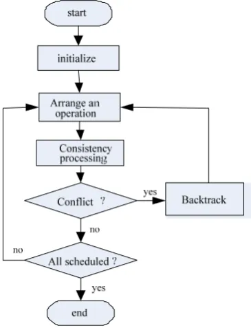
Constraint programming [7] is an effective methodology for solving difficult combinatorial problems by representing them as constraint satisfaction problems (CSPs). A constraint satisfaction problem usually consists of a set of variables, a domain for each variable, and a set of constraints restricting the values that the variables can simultaneously take. Backtracking paradigm is a basic constraint propagation technique used to solve constraint satisfaction problems. The basic operation is to pick one variable at a time, and consider one value in its domain at a time, making sure that the newly picked label is compatible with the instantiated partial solution so far. If the newly picked label violates certain constraints, then an alternative value, if exists, is picked. If no value can be assigned to a variable without violating any constraint, it will backtrack to the most recently instantiated variable. This process
[image:3.595.341.524.104.343.2]continues until a feasible solution is found or all possible combinations of labels have been tried and failed [7]. The procedure of constraint programming with backtracking propagation is presented in Figure 1.
Figure 1 The procedure of constraint programming
B. Discrete particle swarm optimization
Particle swarm optimization (PSO), a population-based optimization approach inspired by the observations of bird flocking and fish schooling, was proposed by Kenndey and Eberhart in 1995 [8]. The basic idea of this approach is to locate the optimal or near optimal solution through cooperation and sharing of information among individuals in the swarm. The swarm is composed of a group of particles in a search space with two important characteristics, namely position and velocity. Each particle represents a potential solution, which flies through the hyperspace and has two essential reasoning capacibilits: the memory of its own best position and the knowledge of the global or its neighborhood’s best position. Particles within the swarm communicate information with each other and adjust their own position and velocity based on the information according to following equations:
1 1( ) 2 2( )
i i i i i
V V c r PX c r G X (15)
i i i
X X V (16) whereXi represents the position of particle i, Vi represents
the velocity of particlei, Pi is the best previously visited
position of particlei, G is the global best position, ω is inertia weight that controls the impact of previous velocity on its current one, which is usually reduced dynamically to decrease the search area : max
max min min
max
( )
t
t t
t
, in
which max and min denote the maximum value and the minimum value of inertial weight respectively, and tmaxis the maximum number of iterations.
[image:3.595.57.281.402.488.2]qualitative distinctions between variables. To meet this demand, a discrete version of particle swarm optimization was proposed [9]. DPSO has two main differences from the original one. First, the particle is composed of binary variables. Second, the velocity must be transformed into the change of probability, which is the chance of the variable taking the value 1. Usually, the transformation is achieved through following sigmoid function.
1 ( )
1 exp( )
i
i s V
V
(17)
Where s V( )i denotes the probability of corresponding bit taking value 1.
In this research, particle kat iteration t can be presented
as ,1 , ,
( ,..., ,..., )
t t t p t P
k k k k
X X X X , where , , ,
( , )
t p t p t p
k k k
X S M ,
,
t p k
S denotes the job production sequence in periodp, and ,
t p k
M denotes workstation assignment of jobs in period p. The best solution found by particle k until iteration t is denoted as ,1 ,
( ,..., )
t t t P
k k k
P P P and the best solution found by the swarm until iterationtis denoted as ,1 ,
( ,..., )
t t t P
g g g
P P P . The velocity of particle k at iterationt can be presented as
,1 , ,
( ,..., ,..., )
t t t p t P
k k k k
V V V V , where , , ,
( , )
t p t p t p
k k k
V VS VM ,
,
t p k
VS denotes the velocity of job production sequence in period p, and t p,
k
VM denotes the velocity of workerstation assignment of jobs in periodp.
To facilitate understanding of the proposed methodology, a job production sequence in a period is used as an example to illustrate the construction of a particle.
In t p,
k
S , , , ,
,1 ,
( ,..., )
t p t p t p
k k k N
S S S ,and , , , ,
, ( , ,1, , ,2,..., , , )
t p t p t p t p
k j k j k j k j N
S s s s .
, , ,
t p k j d
s is binary where it is equal to 1 if job j is in the
th
d positionof the production sequence; otherwise, it is 0. For example, suppose the job production sequence in period 1 is (2, 3, 4, 1,) in a particle. Then ,1 ,1 ,1 ,1
,2,1 ,3,2 ,4,3 ,1,4 1
t t t t
k k k k
s s s s and
all other bits are equal to zero. In t p,
k
VS , , , ,
,1 ,
( ,..., )
t p t p t p
k k k N
VS VS VS and , , , ,
, ( , ,1, , ,2,..., , , )
t p t p t p t p k j k j k j k j N VS vs vs vs . Higher value of ,
, ,
t p k j d
vs means that job jis more likely to be placed in the dthposition in period p, while lower value indicates that it is better to place the job in another position. In each iteration, the velocity is updated according to equation (15), and then converted to the change of probability via the following sigmoid function.
, ,
, , ,
, 1
( ) 1, 2,...,
1 exp( )
t p d
k j t p d p
k j
s vs d N
vs
(18)
where Np is the number of jobs in period p ,
, , , ( k jt p d)
s vs denotes the probability of placing job j in the
th
d position of the production sequence in periodp.
In the iteration process of discrete particle swarm optimization, each particle should be decoded into a complete production schedule. In the job production sequence example, the construction of a job production sequence in period p starts from a null sequence and then places an unscheduled
job j in the dth position from d1 to Np according to
following probability [10]:
' '
, , , ,
, , ,
,
( )
( )
( )
t p d k j t p
k d t p d
k j j U
s vs
q j
s vs
(19)where U is the set of of unscheduled jobs in periodp, and ,
, ( )
t p k d
q j is the probability of placing job jin the dthposition. A complete job production sequence of a period has been constructed when each of the jobs in this period has been assigned to a position.
C. The proposed hybrid algorithm
Step 1. Initialization
Step 1.1 Initialize parameters, particle size K, tmax
Step 1.2 Initialize particles’ positions Xtk and velocities t k
V randomly.
Step 1.3 Evaluate objective function value for each particle. Initialize Pkt
and Pgt
Step 2. Perform iteration process
while(t t max)
Step 2.1 for k1 to K
Update velocity of particle k for p1 to P
Update job production sequence in periodpof particlek
while job production sequence of period p is not empty Pick the first jobj in the production sequence
Update work station assignment of job j
Check consistency
while (not consistent)
Detect critical machine and add to violation set
if there is alternatives of the critical machine change a new assignment
check consistency
else
randomly assign a suitable machine
set it consistent
end-while
calculate production output of jobj in periodp delete this job from the job production sequence
end-while
end-for Update Pkt
end-for
Step 2.2 Update Pgt
Step 2.3 Increment of iteration count t t 1
end-while
Step 3. Report the best solution of the swarm and corresponding objective function value
Particle swarm optimization is an effective algorithm for solving many types of optimization problems. However, if the swarm is going to be in equibrium, the evolution process will be staganeted as time goes on [11]. Constraint programming is specialized for solving problems with hard constraints, but may be inefficient when the feasible search space is very large. Hence, a hybrid algorithm which combines their complementary advantages to improve the search process is proposed in this research. The proposed hybrid algorithm is summarized briefly in Figure 2.
In this research, the planning horizon consists of multi periods. Due to capacity limitations of the various workstations, some jobs may not be finished before their due dates in some periods while some workstations may have remaining capacities in some periods. Hence, it is necessary to make a trade-off among inventory holding cost, subcontracting cost, and workstation utilization. A concept called extra capacity is firstly introduced. The extra capacity of a job in a period is the number of units of the job that can be produced in excess in this period without affecting other scheduled jobs. When a job cannot be finished before its due date in a period and has extra capacity in previous periods, the extra capacity will be utilized to produce it and the inventory is carried to this period. If there is still backlog of this job after utilizing extra capacity, the amount will be subcontracted in order to meet customers’ demand.
In practice, subcontracting cost of a job is usually much higher than its inventory holding cost and manufacturing cost. Hence, in the proposed algorithm, if a job cannot be finished before its due date even after utilizing the extra capacity of previous periods, it will be treated as inconsistency and the critical workstation will be detected to try a new assignment. In addition, the procedure indicates that constraint propagation in this research takes the form of single-level backtracking. When inconsistency occurs, the algorithm will detect the critical resource and check whether this critical resource has any alternatives. If yes, another workstation selected from the alternatives will be assigned to perform the operation; otherwise, the algorithm will not backtrack to the most recently scheduled job and just randomly assign a suitable workstation for it according to DPSO mechanism regardless of consistency, and then continue to schedule the next job until all jobs have been scheduled.
IV. COMPUTATION RESULTS
In this section, the performance of the proposed hybrid algorithm is analysed by comparing the results obtained from solving a set of randomly generated test problems with that of DPSO.
A. Test Problem Set and Parameters
The values of parameters used in the algorithm are as follows. Particle size is 100, maximum number of iterations is 100, maximum inertial weight is 0.8, minimum inertial weight is 0.2. c1and c2are both equal to 2, the velocity of particles is restricted in the range [-4, 4]. Each period contains 30 time slices, the length of which is 300 seconds. There are 3 or 4 operations required for producing each unit
of a job. Each operation has a processing time randomly generated from [20, 40]. The number of units that should be produced (a job) in a period is randomly generated from [50, 80]. Table 2 shows the scheme used to generate the test problem. In the table,( , , , , )p n d s m is used to denote the parameter combination, wherepis the number of periods, nis the number of jobs in each period, ddenotes the due date, sdenotes job subcontracting cost, and mdenots the number of workstations. For example, scheme 1 means that there are 5 periods, the number of jobs in a period is randomly generated from [5, 10], the due date of each job is randomly generates from [ S, S], where α0.4,β0.7, the subcontracting cost of each job per unit is generated from [500, 1000], the number of workstations is 12.
TABLE 2PARAMETER SCHEME
No. Parameter value
1 (5, [5, 10], [0.4, 0.7], [500, 1000], 12) 2 (5, [5, 10], [0.6, 0.9], [500, 1000], 12) 3 (5, [5, 10], [0.4, 0.7], [1000, 2000], 12) 4 (5, [5, 10], [0.6, 0.9], [1000, 2000], 12) 5 (5, [5, 10], [0.4, 0.7], [500, 1000], 20) 6 (5, [5, 10], [0.6, 0.9], [500, 1000], 20) 7 (5, [5, 10], [0.4, 0.7], [1000, 2000], 20) 8 (5, [5, 10], [0.6, 0.9], [1000, 2000], 20) 9 (10, [5, 10], [0.4, 0.7], [500, 1000], 12) 10 (10, [5, 10], [0.6, 0.9], [500, 1000], 12) 11 (10, [5, 10], [0.4, 0.7], [1000, 2000], 12) 12 (10, [5, 10], [0.6, 0.9], [1000, 2000], 12) 13 (10, [10, 15], [0.4, 0.7], [500, 1000], 12) 14 (10, [10, 15], [0.6, 0.9], [500, 1000], 12) 15 (10, [10, 15], [0.4, 0.7], [1000, 2000], 12) 16 (10, [10, 15], [0.6, 0.9], [1000, 2000], 12)
B. Comparison with DPSO
Under each scheme, five test problems are randomly generated. The performances of the hybrid algorithm and DPSO are obtained by averaging the results of running the algorithms five times for each problem. Table 3 shows the performance comparison of the two algorithms after executing both algorithms 100 iterations. In the table, cost diff and time diff are calculated according to equations (20) and (21).
cost of DPSO-cost of hybrid algorithm cost diff=
cost of DPSO (20) CPU time of hybrid algorithm-CPU time of DPSO time diff=
CPU time of DPSO (21)
From Table 2, it is clear that the proposed hybrid algorithm can obtain much better schedule solutions in the sacrifice of longer computational time.
Since the hybrid algorithm needs longer computational time for the same number of iterations. It is necessary to compare the performance of these two algorithms with the same computational time. Table 4 lists the comparison results. In this table, Tpsorepresents the computational time
TABLE 3COMPARISON WITHIN THE SAME ITERATIONS
No. DPSO HYBRID Cost diff Time diff
cost time cost time
1 563218 70 531783 89 5.58% 27.14%
2 529196 87 482444 111 8.83% 27.59%
3 711755 108 578140 143 18.77% 32.41%
4 652706 88 560282 114 14.15% 29.55%
5 372065 79 345057 93 7.26% 17.72% 6 501924 78 486018 88 3.17 12.82%
7 714411 117 614808 140 13.94% 19.66%
8 525589 83 503133 96 4.27% 15.66%
9 1140888 204 1051389 247 7.84% 21.08%
10 1176895 177 1100422 218 6.50% 23.16% 11 1175947 182 1029194 219 12.48% 20.33%
12 1046388 174 927337 206 11.38% 18.39%
13 2724866 568 2460257 793 9.71% 39.61% 14 2711063 510 2431879 709 10.30% 39.02% 15 4435985 620 3646998 867 17.79% 39.84% 16 3784960 629 2960653 890 21.78% 41.49%
TABLE 4COMPARISON WITHIN THE SAME COMPUTATION TIME
No.
Cost diff
1/3Tpso 1/2Tpso 2/3Tpso Tpso
1 6.29% 6.29% 5.89% 5.58%
2 9.46% 9.23% 9.26% 8.54%
3 20.33% 19.68% 18.06% 18.63%
4 13.65% 13.36% 13.53% 14.08%
5 6.40% 6.26% 6.67% 7.26%
6 3.09% 2.56% 3.10% 2.74%
7 14.16% 14.46% 14.27% 13.94%
8 4.53% 4.44% 3.79% 3.96%
9 7.29% 7.44% 7.82% 7.83%
10 6.17% 6.53% 6.70% 6.46%
11 14.46% 13.56% 13.14% 12.47%
12 12.48% 11.82% 11.95% 11.32%
13 9.63% 9.64% 9.51% 9.70%
14 10.13% 10.10% 10.32% 10.11%
15 17.29% 16.99% 17.40% 17.62%
16 21.88% 22.00% 21.80 21.72%
It is clear that the proposed hybrid algorithm has better performance in locating good schedules within the same computational time. Furthermore, the improvement is more obvious when problem size becomes larger, due date becomes tighter, or subcontract cost becomes higher. Hence, it is suitable for solving real industrial problems which usually have large problem size.
V. CONCLUSIONS
This paper focuses on solving the production scheduling problem for virtual cellular manufacturing systems operating under a multi-period manufacturing senario. The objective is to minimize the total manufacturing cost within the entire planning horizon. A new mathematical model has been established to describe the characteristics of a virtual cellular manufacturing system and a hybrid algorithm which combines the advantages of the techniques of constraint programming and discrete particle swarm optimization has been developed to generate effectively the optimal production schedule for the manufacturing system.
Computational experiments using a set of randomly generated test problems demonstrates that the hybrid algorithm can generate better production schedules with the same number of iterations or the same amount of computational times, especially when the size of the problem is large.
ACKNOWLEDGEMENT
The work described in this paper was supported by a grant from the research Grants Council of the Hong Kong Special Administrative Region, China (Project No. HKU 715409E).
REFERENCE
[1] U. Wemmerlov and N. Hyer, “Cellular manufacturing in the US industry: a survey of users,” Int. J. Prod. Res, vol. 27, no. 9, 1989, pp. 1511-1530.
[2] J.R. Drolet, “Scheduling virtual cellular manufacturing systems,” PhD Dissertation, Purdue University, West Lafayette, IN, 1989.
[3] V.R. Kannan and S. Ghosh, “Cellular manufacturing using virtual cells”, Int. J. Op. Prod. Manage, vol. 16, no. 4, 1996, pp. 99-112. [4] S.A. Irani, T.M. Cavalier, and P.H. Cohen., Virtual manufacturing
cells: Exploiting layout design and intercell flows for the machine-sharing problem. Int. J. Prod. Res, 1993, 31(4), pp. 791-810. [5] A. Baykasoglu., Capability-based distributed layout approach for
virtual manufacturing cells. Int. J. Prod. Res., 2003, 41(11), pp. 2597-2618
[6] K.L. Mak, J.S.K. Lau and X.X. Wang, “A genetic scheduling methodology for virtual cellular manufacturing systems: an industrial application,” Int. J. Prod. Res, vol. 43, no. 12, pp. 2423-2450, June 2005.
[7] E.P.K. Tsang, Foundation of Constraint Satisfaction. Academic Press, 1993.
[8] J. Kenndey and R.C. Eberhart, “Particle swarm optimization,” IEEE international conference on neural network, pp. 1942-1948, 1995. [9] J. Kenndey and R.C. Eberhart, “A discrete binary version of the particle
swarm optimization,” The world multiconference on systems, cybernetics and informatics, pp. 4104-4109, 1997.
[10] C.J. Liao, C.T. Tseng, and P. Luarn, “A discrete version of particle swarm optimization for flowshop scheduling problems,” Computers and Operations Research, vol 34, pp. 3099-3111, 2007.