Exponential Penalty Methods for Solving Linear Programming Problems

(1)

Exponential Penalty Methods for Solving Linear

Programming Problems

Parwadi Moengin, Member, IAENG

Abstract—This paper is concerned with the study of the

exponential penalty method for linear programming problems with the essential property that each exponential penalty method is convex when viewed as a function of the multiplier.. It presents some background of the method and its variants for the problem. Under certain assumption on the parameters of the exponential penalty function, we give a rule for choosing the parameters of the penalty function. Theorems and algorithms for the methods are also given in this paper. At the end of the paper we give some conclusions and comments on the methods.

Index Terms—linear programming problems, exponential

penalty method, and penalty parameter.

I. INTRODUCTION

The basic idea in exponential penalty method is to eliminate some or all of the constraints and add to the objective function a penalty term which prescribes a high cost to infeasible points (Wright, 2001; Zboo, etc., 1999). Associated with this method is a parameter , which determines the severity of the penalty and as a consequence the extent to which the resulting unconstrained problem approximates the original problem (Kas, etc., 1999; Parwadi, etc., 2002). Parwadi (2010) proposed a polinomial penalty method for solving linear programming problems. In this paper, we restrict attention to the exponential penalty function. Other exponential barrier functions will appear elsewhere. It presents some background of the methods for the problem. The paper also describes the theorems and algorithms for the methods. At the end of the paper we give some conclusions and comments to the methods.

II.STATEMENT OF THE PROBLEM

Throughout this paper we consider the problem maximize ்ܿ_ݔ

subject to Ax = b

x  0, (1) where A 

R

mn, c, x 

R

n, and b 

R

m. Without loss

of generality we assume that A has full rank m. We assume that problem (1) has at least one feasible solution. In order to solve this problem, we can use Karmarkar’s algorithm and simpelx method (Durazzi, 2000).

Manuscript is submitted on February 7, 2011. This work was granted and supported by the Faculty of Industrial Engineering, Trisakti University, Jakarta.

Parwadi Moengin is with the Department of Industrial Engineering, Faculty of Industrial Technology, Trisakti University, Jakarta 11440, Indonesia. (email: parwadi@hotmail.com, parwadi@trisakti.ac.id).

Parwadi (2010 and 2011) also has introduced a polynomial penalty and barrier methods for solving primal-dual linear programming problems. But in this paper we propose a exponential penalty method as another alternative method to solve linear programming problem (1). In this paper we propose only a procedure for solving a constrained problem. Other procedure associated with exponential penalty method to solve the unconstrained problems will arise in other papers.

II. THE EXPONENTIAL PENALTY FUNCTION

We consider the linear programming stated in (1). The exponential penalty function is given by

)

,

(

x



E

=

c

T

x

+

















m

i

x

b

A

1

)

(

exp

(2)

where   0 is a penalty parameter of the function. The penalty is formed from a sum of exponential of constraint violations and the parameter  determines the amount of the penalty. The basic idea in this method is to eliminate all constraints and add to the objective function a penalty term which prescribes a high cost to infeasible points. Associated with this function is a penalty parameter , which determines the severity of the penalty and as a consequence the extent to which the resulting unconstrained problem approximates the original constrained problem.

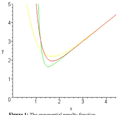
In order to understand the behavior of this function we give the trivial problem

minimize f (x) = x subject to x – 1 = 0,

for which the exponential penalty function is given by

)

,

(

x



E

= x +



exp{





(

x



1 )}

.

Some graphs of

E

(

x

,



)

are given in Figure 1. This figure depicts the one-dimensional variation of the exponential penalty function for three values of , that is  = 2,  = 4 and  = 8. If the solution x * = 1 is compared with the points which minimize

E

(

x

,



)

, it is clear that x * is a limit point of the unconstrained minimizers of

E

(

x

,



)

as   . The y-ordinate of this figure represents

E

(

x

,



)

.

The intuitive motivation for an exponential penalty method is that we seek unconstrained minimizers of

)

,

(

x



(2)

[image:2.595.64.299.49.280.2]

Figure 1: The exponential penalty function

The exponential penalty method for problem (1) consists of solving a sequence of problems of the form

minimize

E

(

x

,



k

)

subject to

x



0

, 3) where

{



k

}

is a penalty parameter sequence satisfying

1

0 _

_

k

_

_

k

for all k, and



k





.

The method depends on the success for sequentially increasing the penalty parameter to infinity. This chapter concentrates on the effect of the penalty parameter. It is easy to show that

E

(

x

,



)

is a convex function for each . The convexity behavior of the exponential penalty function defined by (2) is stated in the following theorem.

Theorem 1 (Convexity)

The exponential penalty function

E

(

x

,



)

defined in (2)is convex in its domain for every   0.

Proof. It is straightforward to prove convexity of

E

(

x

,



)

by using the convexity of

c

T

x

and

















m

i

x

b

A

1

)

(

exp

. Then this theorem is proven.



As a consequence of Theorem 1 we derive the local and global behavior of the exponential penalty function defined by (2) which is stated in the following theorem.

Theorem 2 (Local and global behavior)

(a)

E

(

x

,



)

has a finite unconstrained minimizer in its domain for every   0 and the set Mof unconstrained minimizers of

E

(

x

,



)

in its domain is convex and compact forevery  0.

(b) Any unconstrained local minimizer of

E

(

x

,



)

in its domain is also a global unconstrained minimizer of

)

,

(

x



E

.

Proof. It follows from Theorem 1 that the smooth function

)

,

(

x



E

achieves its minimum in its domain. We then conclude that

E

(

x

,



)

has at least one finite unconstrained minimizer.

By Theorem 1

E

(

x

,



)

is convex, so any local minimizer is also a global minimizer. Thus the set Mof unconstrained minimizers of

E

(

x

,



)

is bounded and closed, because the minimum value of

E

(

x

,



)

is unique, and it follows that Mis compact. Clearly, the convexity of Mfollows from the fact that set of optimal points

E

(

x

,



)

is convex. Theorem 2 is verified. 

Using the results of Theorem 2 we derive the monotonicity behavior of the minimum value of the exponential penalty function

E

(

x

,



)

. To do this, for any

k



 0 we denote

x

k and

E

(

x

k

,



k

)

as a minimizer and minimum value of the problem (3), respectively.

Theorem 3 (Monotonicity)

Let

{



k

}

be an increasing sequence of positive penalty parameters such that



k





as

k





. For sufficiently large k, then



E

(

x

k

,



k

)



is non-increasing.

Proof. Let

x

k and

x

k1 denote global minimizers of the problem (3) for the penalty parameters



kand



k1, respectively. By definition of

x

k and

x

k1 as minimizers and



k 



k1, for sufficiently large k, we have

1



k

T

_x

c

+



k1











_





m

i

i k i

k

_A

_x

_b

1

₍

₎

exp



k

T

_x

c

+



k1











_





m

i

i k i

k

_A

_x

_b

1

₍

₎

exp

, (4a)

k

T

_x

c

+



k1











_





m

i

i k i

k

_A

_x

_b

1

₍

₎

exp



k

T

_x

c

+



k















m

i

i k i

k

_A

_x

_b

1

)

(

exp

, (4b)

k

T

_x

c

+



k















m

i i

k i

k

_A

_x

_b

1

)

(

exp



_c

T

_x

k1

+



k











_





m

i

i k i

k

_A

_x

_b

1

₎

(

exp

. (4c)

(3)

1



k

T

_x

c

+



k1











_





m

i

i k i

k

_A

_x

_b

1

₍

₎

exp



k

T

_x

c

+



k















m

i

i k i

k

_A

_x

_b

1

)

(

exp

.

This means that

)

,

(

_x

k1



k1

E



E

(

x

k

,



k

)

,

as required in the theorem. Hence, the theorem is established. 

Using definition of

E

(

x

k

,



k

)

and Theorem 3, we have 1



k

T

_x

c



_E

(

_x

k1

,



k1

)

_

_E

₍

_x

k

_,



k

₎

. (5) It follows that

f * …

E

(

x

k1

,



k1

)



E

(

x

k

,



k

)

. (6) Let

x

be a limit point of

{

x

k

}

. Since

x

k



0

and

}

0 {

x



R

n

x



is a closed set we obtain that

x



0

.

In another way, by using continuity of function

A

_i

x



b

_i for all i =1,…,m, we see that

k















m

i i

k i

k

_A

_x

_b

1

)

(

exp



0

as

k





₍₇₎

and it is true only if

i k

i

x

b

A





₀

for i =1,…,m, thus,

A

x



b

. Hence,

x

is feasible, and

f * 

c

T

x

.

Using (6), the sequence of



E

(

x

k

,



k

)



of exponential penalty function values is non-increasing and bounded from below, and must converge monotonically from above to a

limit, say g * 

c

T

x

. Suppose that g *  f *. In this case, we define a positive number

  ₂1



g

*



f

*



_.

It follows from

c

T

x

k



c

T

x

that there exists a positive

real number

k

₀ such that for all

k



k

₀,

k

T

_x

c

 g *  . (8) From (7), there exists

k

₁ such that for all

k



k

₁,

k















m

i

i k i

k

_A

_x

_b

1

)

(

exp

 ₂1 _{. (9)}

If we apply (8)(9) and take

k



max

{

k

₀

,

k

₁

}

, the result is

)

,

(

_x

k k

E



=

c

T

x

k

+



k















m

i

i k i

k

_A

_x

_b

1

)

(

exp

 g *  + ₂1 

= g * ₂1. (10)

Taking

k





and using (10), we have

g *  g * ₂1 , that is,

  0,

which contradicts with the assumption that   0. We conclude that g * = f * and

E

(

x

k

,



k

)

 f * as k  , which gives result to the following theorem.

Theorem 4 (Convergence of exponential penalty function)

Let

{



k

}

be an increasing sequence of positive penalty parameters such that



k





as

k





. Let

{

x

k

}

is a sequence of the minimizer of the problem (3) associated with



k. Then

(a)

c

T

x

k



f

*

as k  . (b)

E

(

x

k

,



k

)

 f * as k  . 

III. ALGORITHM

The implication of this theorem is remarkably strong. For any linear programming, the exponential penalty function has a finite unconstrained minimizer for every value of the penalty parameter, and every limit point of a minimizing sequence for the barrier function is a constrained minimizer of a problem (1). Based on the Theorem 4 we construct an algorithm for solving problem (1).

Algorithm 1

Given Ax = b,



1  0, the number of iteration N and   0.

1. Choose

x

1 

R

n such that A

x

1 = b and

x

1  0. 2. If the optimality conditions are satisfied for problem

(1) at

x

1, then stop, else go to Step 3.

3. Compute

E

(

x

1

,



1

)



min

(

,

1

)

0





E

x

and the

minimizer

x

1.

4. Compute

E

(

x

k

,



k

)



min

E

(

x

,

k

)

x0



, the

minimizer

x

k and



k

:



10 

k1 for k = 2.

5. If 

x

k



x

k1   or 

E

(

x

k

,



k

)

–

)

,

(

_x

k1



k1

E

   or k = N then stop, else k  k + 1 and go to Step 4. 

(4)

IV. INTERIORPOINT ALGORITHM

This section reviews the interiorpoint algorithm called Karmarkar’s algorithm for finding a solution of linear programming problem. The step of this algorithm can be summarized as follows for any iteration (Parwadi, 2011).

Step 1. Given the current initial trial solution

(

x

₁

,

x

₂

,...,

x

_n

)

, set















n

x

D

0

0 .

.

0 ...

0

0 ...

0

0 ...

0

3 2 1

.

Step 2. Calculate

A

~



AD

and

c

~



Dc

.

P



I



A

~

T

(

A

~

A

~

T

)

1

A

~

and

c

_p



P

c

~

.

Step 4. Identify the negative component of

c

_p having the largest absolute value, and set  equal to this absolute value. Then calculate





T _p

c

x









1

1 ...

1 ~

_,

where  is a selected constant between 0 and 1.

x



D

x

~

as the trial solution for the next iteration (step 1). (If this trial solution is virtually unchanged from the preceding one, then the algorithm has virtually converged to an optimal solution, so stop.)

V. NUMERICAL EXAMPLES

This section we give five examples to test the Algoirthm 1 and we compare the results with Karmarkar’s algorithm. Consider the following problems (Parwadi, 2010).

Example 1.

Minimize

f



2 x

₁



5 x

₂



7 x

₃ subject to

x

₁



2 x

₂



3 x

₃



6

,

0 

j

x

, for j = 1, 2, 3.

Example 2.

Minimize

f



0 .

4 x

₁



0 .

5 x

₂ subject to

0 .

3 x

1



0 .

1 x

2



2 .

7

,

0 .

5 x

₁



0 .

5 x

₂



6

,

x

_j



0

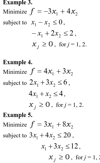
, for j = 1, 2.

Example 3.

Minimize

f





3 x

₁



4 x

₂ subject to

x

1



x

2



0

,



x

₁



2 x

₂



2

,

x

_j



0

, for j = 1, 2.

Example 4.

Minimize

f



4 x

₁



3 x

₂ subject to

2 x

₁



3 x

₂



6

,

4 x

₁



x

₂



4

,

x

_j



0

, for j = 1, 2.

Example 5.

Minimize

f



3 x

₁



8 x

₂ subject to

3 x

₁



4 x

₂



20

,

x

₁



3 x

₂



12

,

0 

j

[image:4.595.300.462.65.329.2] [image:4.595.47.257.162.372.2]

x

, for j = 1, 2.

Table 1 Algorithm 1and Karmarkar’s Algorithm test statistics

Problem No.

Algorithm 1 Karmarkar’s Algorithm Total

Iterations

Time (Secs.)

Total Iterations

Time (Secs.) 1.

2. 3. 4. 5.

11 8 10 12 15

7.6 5.9 8.9 10.9 11.2

16 19 19 12 18

3.6 3.7 3.7 2.8 3.8

Table 1 reports the results of computational for Algorithm 1 and Karmarkar’s Algorithm. The first column of Table 1 contains the example number and the next two columns of each algorithm in this table contain the total iterations and the times (in seconds) of each algorithm. Table 1 also shows that in terms of the number of iterations required to complete the fifth numerical examples, the Algorithm 1 is better than Karmarkar’s Algorithm, but in terms of completion time required to complete the five numerical examples shows that Karmarkar’s algorithm looks better than Algorithm 1. This can be explained that in the proposed approach using an exponential function that generally require a longer time than use a polynomial function as in Karmarkar's algorithm.

VI. CONCLUSION

(5)

solution of problem (1) as the penalty parameter converges to infinity. Moreover, the minimizers of exponential penalty functions converge from the right to the minimizer of problem (1). The algorithm for this method ia also given in this paper. We also note the important thing of these methods which do not need an interior point assumption.

REFERENCES

[1] Durazzi, C. (2000). On the Newton interior-point method for nonlinear programming problems. Journal of Optimization Theory and Applications. 104(1). pp. 7390.

[2] Kas, P., Klafszky, E., & Malyusz, L. (1999). Convex program based on the Young inequality and its relation to linear programming. Central European Journal for Operations Research. 7(3). pp. 291304.

[3] Parwadi, M., Mohd, I.B., & Ibrahim, N.A. (2002). Solving Bounded LP Problems using Modified Logarithmic-exponential Functions. In Purwanto (Ed.), Proceedings of the National Conference on Mathematics and Its Applications in UM Malang. pp. 135-141.

[4] Parwadi, M. (2010). Polynomial penalty method for solving linear programming problems. IAENG International Journal of Applied Mathematics. 40(3), pp. 167-171.

[5] Parwadi, M. (2011). Some algorithms for solving primal-dual linear programming using barrier methods. International Journal of Mathematical Archive. 2(1), pp. 108-114.

[6] Parwadi, M. (2011). Polynomial barrier method for solving linear programming problems International Journal of Engineering and Technology. 11(1), pp. 118-129.

[7] Wright, S.J. (2001). On the convergence of the Newton/log-barrier method. Mathematical Programming, 90(1), 71100.