Assessment of Power Quality Events by Empirical
Mode Decomposition based Neural Network
M Manjula, A V R S Sarma, Member, IEEE
Abstract—The paper presents assessment of various power
quality events based on Empirical Mode Decomposition (EMD) with Hilbert Transform (HT). EMD method decomposes the signal into waveforms modulated in both amplitude and frequency. The oscillatory modes embedded in the signal are extracted by employing sifting process. These oscillatory modes are called Intrinsic Mode Functions (IMFs). The magnitude plot of the Hilbert Transform of the first IMF correctly detects the event. The characteristic features of the first three IMFs of each disturbance are used as inputs to Probabilistic Neural Network (PNN) for identification of the disturbances. Simulation results show that EMD method can effectively classify the power quality disturbances.
Keywords-Empirical mode decomposition, intrinsic mode
functions, hilbert transform, power quality events, probabilistic neural network.
I. INTRODUCTION
ower Quality problem has become a major issue both for industries and utility. Any variation in magnitude and frequency of the voltage or current waveform is defined as power quality. Some of the power quality problems are the voltage sag, swell, interruption, flicker, and transients etc. which cause mal operation or failure of power equipment. To improve the power quality or to find a solution to mitigate them, this involves having a powerful tool or method which can detect, localize and classify the power quality disturbances. This paper aims at classification of various power quality disturbances. The rms magnitude of voltage supply is used in the power quality standards for detection and characterization of voltage events [1]. The method is simple and easy to implement but it does not give information about the phase angle or the point on wave where the event begins [2]. However, rms method has important limitations in the detection and estimation of magnitude and duration of voltage events. A simple way to analyze any signal is by Fourier Transform [3] (FT). It provides only frequency content; therefore this method is applicable for stationary signals.
Manuscript received March 06, 2012; revised March 31, 2012.
M. Manjula is with the Department of Electrical Engineering, University College of Engineering, Osmania University, Hyderabad, 500 007 India (phone: +919948915758; e-mail: manjulamane04@ yahoo.com). A.V.R.S.Sarma is with the Department of Electrical Engineering, University College of Engineering, Osmania University, Hyderabad, 500 007 India ( phone: +919246296940; e-mail: avrs2000@ yahoo.com).
Short Time Fourier Transform (STFT) is proposed [4-5] which maps a signal into a two dimensional function of time and frequency. The disadvantage of STFT is that the size of the window chosen is fixed. This makes a compromise between time and frequency resolution. The wavelet analysis [6-10] on other hand represents a windowing technique with variable regions to overcome the above deficiency. It provides a unified methodology to characterize power quality events by decomposing the signal into time and frequency resolution. So, wavelet function is localized both in time and frequency, yielding wavelet coefficients at different scales. The draw back of wavelet transform is choice of window function and another disadvantage is the use of ranges of frequency. The S-transform [11] on the other hand is an extension to wavelet transform and is based on moving and scalable localizing Gaussian window.
The paper employs Empirical Mode Decomposition (EMD), introduced by Huang [12], together with Hilbert transform for extracting instantaneous amplitude and frequency from multi component non stationary signals. These mono component signals are called the Intrinsic Mode Functions. The advantage of this method is that it does not require predetermined set of functions as in previous methods but allows projection of a non stationary signal onto a time frequency plane using a mono component signals, from the original signal thus making it adaptive in nature.
The rest of the paper is organized as follows: Section II gives introduction to EMD and Hilbert transform. Section III presents the detection capability of the proposed method for power quality events. In section IV gives the introduction of PNN. Section V the simulation results based on the EMD method are discussed. Finally section VI gives the conclusions.
II. EMPIRICAL MODE DECOMPOSITION
Empirical mode decomposition is a method which extracts mono component and symmetric components from the non linear and non stationary signals by sifting process. The name, sifting, indicates the process of removing the lowest frequency information until only the highest frequency remains. The key feature of EMD is to decompose a signal into so called intrinsic mode functions. These Intrinsic Mode Functions extracted from the original signal are mono component composing of single frequency or narrow band of frequencies. An IMF is defined as an oscillating wave, if it satisfies the following two conditions:
1. For a data set, the number of extreme and the number of zero crossings must either be equal or differ at most by one.
2. At any point, the mean value of the envelope defined by the local maxima and the local minima is zero.
The algorithm for extracting an IMF by sifting process is given below:
Step1: The upper and the lower envelopes are constructed by connecting all the maxima and all the minima with cubic splines, respectively.
Step 2: Take the mean of the two envelopes and let it be defined as m(t). Subtract the mean m(t) from the original signal x(t) to get a component h1(t),
Where
h
1(
t
)
x
(
t
)
m
(
t
)
(1)
Step 3: If h1(t) satisfies the two conditions of IMFs , then h1(t) is the first intrinsic mode function else it is treated as the original function and steps (1) - (3) are repeated to get component h11(t) such that
h
11(
t
)
h
1(
t
)
m
1(
t
)
(2)
Step 4: The above sifting process is repeated k times, h1k(t) becomes an first IMF and be known as IMF1.
Separate IMF1 from x(t) and let it be r1(t), such that
r
1(
t
)
x
(
t
)
h
1k(
t
)
(3) (3)
Step 5: Now taking the signal r1(t) as the original signal and repeating the steps (1)-(4) second IMF is obtained.
The above procedure is repeated n times and such n IMFs are obtained. The stopping criterion for the decomposition process is when rn(t) becomes a monotonic function from which no more IMF can be extracted.
A. Hilbert Transform
The Instantaneous frequency of each IMF is calculated by using the Hilbert Transform. The Hilbert Transform of a real valued time domain signal x(t) is another real valued time domain signal, denoted by
x
ˆ
(t), such that z(t) = x(t) + jx
ˆ
(t) is an analytic signal. From z(t), one can define a magnitude function A(t) and a phase function θ(t), where the first describes the envelope of the original function x(t) versus time and θ(t) describes the instantaneous phase of x(t) versus time.In terms of x(t) and
x
ˆ
(t),
() ˆ ()
)
(t x2 t jx2 t 12
A (4)
) (
) ( ˆ tan )
( 1
t x
t x t
(5)
and the “instantaneous frequency” is given by:
) (
) ( ˆ tan 2
1 1
0
t x
t x t f
(6)
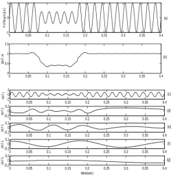
The above algorithm is implemented on a voltage sag waveform. Fig. 1(a) shows the waveform of voltage sag, (b) the magnitude plot of Hilbert transform of IMF1 and (c)- (g) corresponding intrinsic mode functions of sag in voltage.
0 0.05 0.1 0.15 0.2 0.25 0.3 0.35 0.4 -1
0 1
V
o
lt
age
(p
u)
0 0.05 0.1 0.15 0.2 0.25 0.3 0.35 0.4 0
0.5 1 1.5
IM
F
-H
(a)
(b)
0 0.05 0.1 0.15 0.2 0.25 0.3 0.35 0.4
-2 0 2
IM
F
1
0 0.05 0.1 0.15 0.2 0.25 0.3 0.35 0.4
-0.2 0 0.2
IM
F
2
0 0.05 0.1 0.15 0.2 0.25 0.3 0.35 0.4
-0.1 0 0.1
IM
F
3
0 0.05 0.1 0.15 0.2 0.25 0.3 0.35 0.4
-0.1 0 0.1
IM
F
4
0 0.05 0.1 0.15 0.2 0.25 0.3 0.35 0.4
-0.2 0 0.2
time(sec)
IM
F
5
(c)
(d)
(e)
(f)
(g)
Fig. 1(a). Waveform of voltage sag ,(b) magnitude plot of hilbert transform of IMF1, (c) – (g) IMF1 to IMF5.
III. PQ EVENTS ASSESSMENT BY EMD METHOD
The detection of various power quality events based on Empirical Mode Decomposition method with Hilbert transform. The magnitude plot of the Hilbert transform of the first IMF obtained by sifting process gives the information of the magnitude and phase of the frequency content of the signal and is used to detect the disturbance. The power quality disturbances like Voltage Sag, Voltage Swell, Harmonic, Transient, Sag with harmonic, Swell with harmonic, Outage, Flicker, Notch and Spike are generated using MATLAB software.
A. Voltage swell
Fig. 2(a) shows the case for voltage swell signal. The event occurs from 0.14 to 0.3sec for about 8 cycles with 1.5pu magnitude. Fig. 2(b) shows the magnitude plot of Hilbert transform of the IMF1 which correctly detects the swell event.
0 0.05 0.1 0.15 0.2 0.25 0.3 0.35 0.4
-2 0 2
V
ol
tage
(pu)
0 0.05 0.1 0.15 0.2 0.25 0.3 0.35 0.4
0.5 1 1.5 2
IM
F
-H
(a)
(b)
[image:2.595.311.561.55.311.2] [image:2.595.312.552.618.709.2]B. Harmonic
Fig.3 (a) shows the waveform of harmonic signal. The signal contains of pure sine of 1pu, 0.14pu of 3rd harmonic, 0.12pu of 5th harmonic, 0.11pu of 7th harmonic. Fig. 3(b) shows the IMF1 which gives the presence of harmonics. Fig.3(c) and (d) shows the waveform of harmonic content (IMF1-IMF2).
0 0.05 0.1 0.15 0.2 0.25 0.3 0.35 -2
-1 0 1 2
V
ol
tage(
pu)
0 0.05 0.1 0.15 0.2 0.25 0.3 0.35 0
0.1 0.2 0.3 0.4
IM
F
-H
(a)
(b)
0 0.05 0.1 0.15 0.2 0.25 0.3 0.35
-0.4 -0.2 0 0.2 0.4
IM
F
1
0 0.05 0.1 0.15 0.2 0.25 0.3 0.35
-1 -0.5 0 0.5 1
time(sec)
IM
F
2
(c)
(d)
Fig. 3(a). Waveform of voltage harmonics ,(b) magnitude plot of hilbert transform of IMF1, (c) - (d) IMF1- IMF2.
C. Sag with harmonic
Here Fig. 4(a) shows the case of sag with harmonics. The signal contains 1pu pure sine wave, 0.12pu 3rd harmonic, 0.11pu 5th harmonic, 0.10pu 7th harmonic and sag of 0.7pu magnitude is introduced from 0.06 to 0.15sec. Fig. 4(b) shows the magnitude plot of Hilbert transform of the IMF1 which rightly detects the sag event and presence of harmonics.
0 0.05 0.1 0.15 0.2 0.25 0.3 0.35 0.4
-1 -0.5 0 0.5 1
V
o
lt
ag
e(
pu)
0 0.05 0.1 0.15 0.2 0.25 0.3 0.35 0.4
0 0.1 0.2 0.3 0.4
IM
F
-H
(a)
(b)
Fig. 4(a). Waveform of voltage sag with harmonics ,(b) magnitude plot of hilbert transform of IMF1.
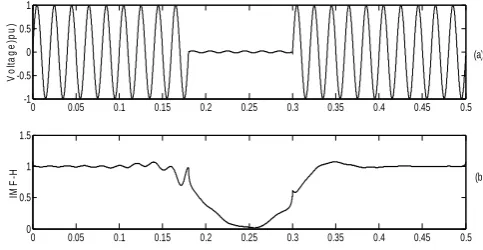
D. Outage and Flicker
Here the occurrence of outage for about 6 cycles is shown in Fig. 5(a). Fig. 5(b) shows the magnitude plot of HT where the voltage goes to zero during that period.
The phenomenon of flicker is generated by combination of pure sine of 1pu magnitude and 0.13pu, 10Hz signal as shown in Fig. 6(a). Fig. 6(b) shows the presence of the low frequency signal. Fig. 8(c) shows the IMF1.
0 0.05 0.1 0.15 0.2 0.25 0.3 0.35 0.4 0.45 0.5 -1
-0.5 0 0.5 1
V
o
lt
age
)p
u)
0 0.05 0.1 0.15 0.2 0.25 0.3 0.35 0.4 0.45 0.5 0
0.5 1 1.5
IM
F
-H
(a)
(b
Fig. 5(a). Waveform showing outage ,(b) magnitude plot of hilbert transform of IMF1.
0 0.05 0.1 0.15 0.2 0.25 0.3 0.35 0.4 0.45 0.5
-2 0 2
V
ol
tage(
pu)
0 0.05 0.1 0.15 0.2 0.25 0.3 0.35 0.4 0.45 0.5
0.5 1 1.5
IM
F
-H
0 0.05 0.1 0.15 0.2 0.25 0.3 0.35 0.4 0.45 0.5
-2 0 2
time(sec)
IM
F
1
(a)
(b)
(c)
Fig. 6(a). Waveform of voltage flicker ,(b) magnitude plot of hilbert transform of IMF1, (c) IMF1.
E. Notch and Spike
Fig. 7(a) shows the case of signal having 2 notches/cycle. The magnitude plot of the IMF1 clearly detects the notches as shown in the Fig. 7(b).
Fig. 8(a) shows the case of signal having spike for 0.25msec with magnitude of 1.3pu. The magnitude plot of the IMF1 clearly detects the spike as shown in the Fig. 8(b).
The first three IMFs are considered for the feature extraction. The following three features are (1) Energy distribution, (2) Standard deviation of the amplitude and (3) Standard deviation of the phase. Thus, we have nine features from the three IMFs from each disturbance.
0 0.05 0.1 0.15 0.2 0.25 0.3 0.35 0.4 0.45 0.5
-1 -0.5 0 0.5 1
Vol
tag
e(
p
u)
0 0.05 0.1 0.15 0.2 0.25 0.3 0.35 0.4 0.45 0.5
0 0.2 0.4 0.6 0.8
IM
F
-H
(a)
(b)
[image:3.595.308.550.58.183.2] [image:3.595.50.291.148.338.2] [image:3.595.311.554.232.364.2] [image:3.595.51.285.500.609.2] [image:3.595.307.552.584.709.2]0 0.05 0.1 0.15 0.2 0.25 0.3 0.35 0.4 0.45 0.5 -1
0 1 2
V
ol
tag
e(
p
u)
0 0.05 0.1 0.15 0.2 0.25 0.3 0.35 0.4 0.45 0.5
0 0.1 0.2 0.3 0.4
IM
F
-H
(a)
(b)
Fig. 8(a). Waveform showing spike ,(b) magnitude plot of hilbert transform of IMF1.
IV. PROBABILISTIC NEURAL NETWORK
The Probabilistic Neural Network (PNN) is a supervised neural network that is widely used in the area of pattern recognition. The fact that PNNs offer a way to interpret the network’s structure in terms of probability density functions (PDF) is an important merit of this type of networks. The following features are distinct from those of other networks in the learning processes.
It is implemented using the probabilistic model, such as Bayesian classifiers.
A PNN is guaranteed to converge to a Bayesian classifier provided that it is given enough training data.
No learning processes are required.
No need to set the initial weights of the network. No relationship between learning processes and
recalling processes.
The differences between the inference vector and the target vector are not used to modify the weights of the network.
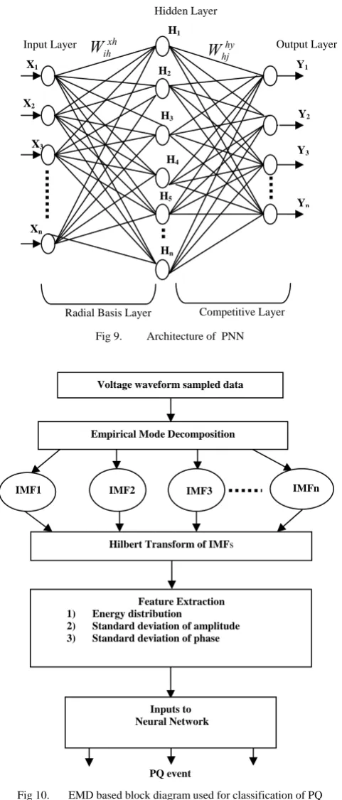
The standard training procedure for PNNs requires a single pass over all to the patterns of the training set. This characteristic renders PNNs faster to train suitable for classification of power system faults. The architecture of PNN is composed of radial basis layer and competitive layer as shown in Fig.9.
The probabilistic neural network (PNN) is a supervised neural network that is used for classification.
Multi-layer neural network with three layers – input, hidden and output layers is also implemented. The input layer has 3 nodes represented by features extracted by EMD; hidden layer has 11 nodes, while output layer has 10 nodes representing 10 classes of disturbances: voltage sag, voltage swell, interruption and harmonic distortion etc.
In this paper, an approach of probabilistic neural network is explored to classify power quality problems. The performances of EMD based PNN and MLNN are compared in the next section.
Fig.10 shows the block diagram for classification of power quality events using probabilistic neural network and multilayer neural network.
[image:4.595.52.291.59.182.2]Fig 9. Architecture of PNN
Fig 10. EMD based block diagram used for classification of PQ
disturbances.
V. RESULTSANDDISCUSSION
Ten types of PQ disturbances are taken for case study as S1-Sag; S2-Swell; S3-Harmonic; S4-Transient; S5-Sag with Harmonic;S6-Swell with Harmonic;S7-Outage; S8-Flicker; S9- Notch and S10-Spike. Simulations are performed to generate about 1500 signals, 500 data sets are used for training the MLNN classifier and 1000 are used for testing. The classification result using the PNN method is shown in Table I and MLNN is shown in Table II. The application of EMD decomposes the disturbance signal into number of
PQ event
Voltage waveform sampled data
Empirical Mode Decomposition
IMF1 IMF3 IMFn
Hilbert Transform of IMFs
Feature Extraction
1) Energy distribution
2) Standard deviation of amplitude
3) Standard deviation of phase
Inputs to Neural Network IMF2
Output Layer Input Layer
X1
X2
X3
Xn
Hidden Layer
Y1
Y2
Y3
Yn
H1
H2
H3
H4
H5
Hn
Radial Basis Layer Competitive Layer
xh ih
W
hyhj
[image:4.595.308.549.69.633.2]IMFs. The number of IMFs for a given disturbance depends upon the severity of distortion and magnitude of harmonic content. The first IMF magnitude plot of Hilbert transform provides the true instantaneous amplitude change in case of sag and swell.
It is found that by adopting the proposed technique, the signal features can be correctly identified for a disturbance like notch and spike which occurs for a very small duration of time ,ie few milliseconds . In the case of harmonics and flicker, as IMFs are mono component signals extracted from the disturbance, they directly give the information of the frequency content of the signal. As previously mentioned, EMD is a sieving process and the first IMF represents the finest scale of oscillation of the signal. Hence, an event like notch and spike which occurs for milliseconds of time can be classified very accurately by this methodology.
VI. CONCLUSIONS
In this paper EMD with Hilbert transform is used to analyze and classify the power quality disturbances. EMD method was able to decompose different modes of oscillations from the original signal into mono component signals to extract instantaneous frequency information for each mode of oscillation thus, making it a better method in assessing power quality events. The results show the superiority of the method in correctly classifying the disturbances. Hence the proposed method is suitable for classification of non-stationary signals.
REFERENCES
[1] Emmanouil Styvaktakis, Irene Y. H. Gu , Math H. J. Bollen,
“Voltage Dip Detection and Power system transients”,IEEE Trans.
Power Engg. Society Summer Meeting, Vol. 1, 15-19 July 2001, pp. 683-688
[2] Math H. J. Bollen, “Understanding Power Quality Problems :
Voltage Sags and Interruptions” ,IEEE Press.
[3] A. Flores, “State of art in the classification of power quality events,
an overview,” in Proc. 10th Int. Conf. Harmonics Quality Power,
2002, vol.1, pp.17-20.
[4] Y. H. Gu and M. H. J. Bollen, “Time-frequency and time-scale
domain analysis of voltage disturbances,” IEEE Trans. Power Delivery, vol. 15, no.4 pp. 1279-1284, October 2000.
[5] F. Jurado, N. Acero, and B. Ogayar, “Application of signal
processing tools for power quality ,” in Proc. Canadian Conf. Electrical and Computer Engineering, May 2002, vol.1, pp 82-87.
[6] S. Santoso, W. M. Grady, E. J. Powers, J. Lamoure, and S. C. Bhatt,
“Characterization of distribution power quality events with Fourier and Wavelet transforms,” IEEE Trans. Power Delivery , vol.15, No.1, pp. 247-245, January 2000.
[7] Z. L. Gaing, “Wavelet based neural network for power disturbance
recognition and classification,” IEEE Trans. Power Delivery, vol.19, No.4, pp.1560-1568, Oct. 2004.
[8] M.Gaouda, M.M.A.Salama and M.R.Sultan, A.Y.Chikhani, "Power
Quality Detection and Classification Using Wavelet Multiresolution Signal Decomposition”, IEEE Transactions on Power Delivery, Volume 14, Issue 4 October 1999, pp. 1469-1476.
[9] H. Amaris, C. Alvarez, M. Alonso, D. Florez, T. Lobos, P. Janik, J.
Rezmer, Z. Waclawek,” Application of advanced signal processing
methods for accurate detection of voltage dips,’ 13th International
Conference on Harmonics and Quality of Power, ICHQP
2008,Wollongong,Australia, pp.6 28th September 2008.
[10] Haibo He,and Janusz A. Starzyk, A Self-Organizing Learning Array
System for PowerQuality Classification Based on Wavelet
Transform, IEEE Transactions on Power Delivery, Volume 21, Issue
1 January 1999.
[11] S. Mishra, C. N. Bhende, and B. K. Panigrahi, “Detection and
classification of power quality using S-transforms and probabilistic neural network, “IEEE Transactions on Power Delivery, Vol 23, Issue 1, January 2008, pp.280-287.
[12] N.E. Huang, Z. Shen, S.R. Long, M.C. Wu, H.H. Shih, Q. Zheng,
[image:5.595.40.554.635.756.2]N.C. Yen, C.C. Tung, H.H. Liu, The empirical mode decomposition and hilbert spectrum for nonlinear and non stationary time series analysis, Proceedings of the Royal Society, London, Series A 454, 903-995, 1998.
Table I
Percentage classification accuracy of PNN
Signal Sag Swell Harmonics Transient Sag with
Harmonics
Swell with
Harmonics Outage Flicker Notch Spike
Sag 100
Swell 100
Harmonics 98 2
Transient 5 95
Sag with Harmonics 3 97
Swell with Harmonics 5 95
Outage 100
Flicker 2 98
Notch 100
Spike 100
Classification Accuracy: 98.3%
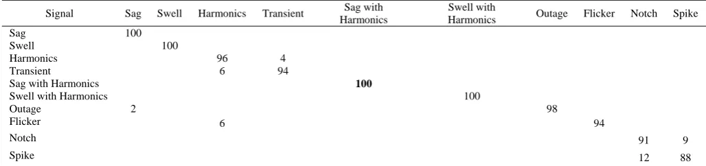
Table II
Percentage classification accuracy of MLNN
Signal Sag Swell Harmonics Transient Sag with
Harmonics
Swell with
Harmonics Outage Flicker Notch Spike
Sag 100
Swell 100
Harmonics 96 4
Transient 6 94
Sag with Harmonics 100
Swell with Harmonics 100
Outage 2 98
Flicker 6 94
Notch 91 9
Spike 12 88