Analyzing the Effects of Graph Construction
Methods on Image using Graph Signal Processing
S.K.Pavithra1, S.Senthilkumar2
1PG Scholar, 2Associate Professor, GRT Institute of Engineering and Technology, Tiruttani, Chennai
Abstract: Graph signal Processing is fast developing area in signal processing domain, especially processing large signal data, because graphs are having strength to represent large datasets with ease and also it is natural way of representing the signals on irregular domain. In this paper, we have discussed the effects of the various graph construction methods on image processing using Graph Fourier Transform and also through the image de-noising application. The analysis shows that the KNN graph is more suitable method to represent an image as well as for image de-noise application.
Keywords: Graph Fourier Transform, Graph Filtering, Regional Graph, Gaussian Graph, E-Ball NN Graph.
I. INTRODUCTION
In the recent years, there have been significant progress in the development of theory, tools, and applications of graph signal processing. Graph signal processinghasbecomes first consideration in numerous practical cases where the signal domain is not a set of equidistant instants in time or a set of points in space on a regular grid. For example, sensor networks deployed to measure physical entities like temperature and solar radiation, traffic volumes in transportation networks, brain activities in biological networks. Online social networks such as whatsapp, Linkedin,Twitter, Facebook that turned into a significant means of communication. 3D depth cameras used to capture dynamic 3D scenes in emerging applications such as gaming, immersive communication and virtual reality. Such data is usually very complex because of its extremely high-dimensional and occupies a large amount of storage space, irregularly structure and the data and the structure may be generated by different sources of information [1].
The representation, analysis, and compression of such data is a challenging task that requires the development of new tools like Graph signal processing that can identify and properly exploit data structures. The data domain, in these cases, is defined by a graph. The graph consists of vertices, where the data values are defined / sensed, and the edges connecting these vertices. Graph exploits the fundamental relations among the data based on their relevant properties. Processing of signals whose sensing domains are defined by graphs resulted in graph data processing as an emerging field [1][2] in big data signal processing today. This is a big step forward from the classical time (or space) series data analysis.
II. GRAPH CONSTRUCTIONS FOR IMAGES
Graph construction is a crucial step in graph signal processing. Because it influence the results of various graph signal processing methods [3]. Suitability of several approaches of graph construction based on the popular k-nearest neighbors method (kNN) for image processing are analyzed in this article.
A. k- Nearest Neighborhood Graph:
Constructing a graph with k-nearest neighbors (k-NN)[4],[5] is a popular method. In this method, an edge is set between two vertices if vertex vj is in k-NN of vertex vi. Each vertex has its own k-nearest neighbors. Consequently, the graph is a directed graph.
It is worth noting that constructing such a graph requires calculating all pairwise distances and ordering these values on each vertex, and these operations lead to high computational costs.
The choice of k is crucial to have a good performance. A small k makes the graph too sparse or disconnected so that the hill-climbing method frequently gets stuck in local minima. Choosing a big k gives more flexibility during the runtime, but consumes more memory and makes the offline graph construction more expensive.
B. E-ball Graph:
This is same as k-NN graph except that contains all the vertices connected to other vertices if it’s pairwise distances is within the threshold value defined by the user [6].
A Gaussian kernel is a kernel with the shape of a Gaussian (normal distribution) curve. This method of graph construction also same like k-NN graph construction method but uses Gaussian kernel function [7][8] defined as below to find the pairwise distances instead of Euclidean distances
D. Region Graph
Any segmentation of an image can be associated with a region adjacency graph [9]. Specifically, given a graph G = {V, E} where each node is identified with a pixel, a partition into R connected regions V1∪V2∪. . .∪VR = V, V1∩V2∩. . .∩VR = ϕ may be
identified with a new graph ˜G = {˜V,˜E } where each partition of V is identified with a node of ˜V, that is, Vi Є ˜V. A common method for defining ˜E is to let the edge weight between each new node equal the sum of the edge weights connecting each original node in the sets, that is, for edge eijЄE.
Each contiguous Vi is called a superpixel. Superpixels are an increasingly popular trend in computer vision and image processing.
III. GRAPH FOURIER TRANSFORM AND GRAPH FILTERING
A. Graph Fourier Transform:
Assume that the spectral decomposition, or eigen decomposition of the graph shift matrix A is
A = VΛV-1
where Λ = diag(λ0,… λN-1) is the diagonal matrix of N distinct eigenvalues and V is the matrix of corresponding eigenvectors.1 The
eigenvalues of A represent the graph frequencies and the eigenvectors form a basis of spectral components. The graph Fourier transform corresponds to the expansion of a graph signal into the basis of spectral components and can be written as
where F = V-1 is the graph Fourier matrix. Respectively, the inverse graph Fourier transform reconstructs the signal from its
frequency representation as
x = F-1x̂ B. Graph Filtering:
A graph filter is a system that takes a graph signal as an input and produces another graph signal as an output. The most elementary nontrivial graph filter, graph shift, replaces the signal value at a node with a weighted linear combination of values at its neighbors. This operation is written as
y = Ax
Every linear, shift-invariant graph filter is a polynomial in the graph shift
and its output is given by the matrix-vector product
y = h(A) x
IV. EXPERIMENTS AND ANALYSIS
Standard image set of size 32x32 is chosen for analysis to reduce the processing time by the matlab. Matlab tool: GSPBOX developed at the signal processing Laboratory LTS2 of EPFL [14] is used for graph construction, application of GFT on the constructed graph and de-nosing by graph filter.
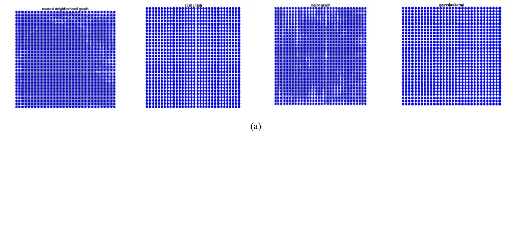
To analyses the effect of the graph construction on the image using graph signal processing, we have taken up Graph Fourier Transform (GFT) of the graphs of the image. Figure 2 (a) show the various graphs constructed from the image shown in figure 1 and figure 2(b) show the respective graph signals. Figure 3 show the graph spectrum of the respective graph signals shown in figure 2(b). Given a large graph it would be useful to be able to take a small snapshot that can concisely capture information about the graph. one of the most useful ways of doing this has been by studying the various spectra of matrices (i.e., the eigenvalues of the matrices) that can be associated with the graph. By looking at these eigenvalues it is possible to get information about a graph that might otherwise be difficult to obtain. The study of the relations between eigenvalues and structures in graphs is the heart of spectral graph theory. Comparing the eigenvalues, we see that they can be quite different. In general it will make a big difference as to which spectrum is used, and some results which might hold for one spectrum may not hold for another.
From figure 3.(a) and figure 4 we can be understood that most of the eigen values of kNN graph are very smaller compare to the one largest eigen values and also have different number of multiplicity, this shows that the graph is not complete graph as each node connected to the different number of nodes i.e each node have different degrees. In figure 3.(b) and figure 4 we can see that most of the eigen values of e-ball graph are almost same and close to zero ,this reflect that each node in the graph has less number of edges or no edges. This is mainly due to the selection of the proper value for ball radius for nearest neighborhood connection. For suitable value of ball radius one should have the knowledge of the image otherwise this method of graph construction will not reflect the structure underline the image properly. Figure 3.(c) and figure 4 shows that the eigen values of region graph are same like eigen values of kNN graph except that the eigen values are very small and not much varied ,this reflect that the region graph are smoother than therkNN graph because of this graph signal of region graph is not exactly replicate the image. This is happened due to grouping of the image pixel to form the super pixel. In figure 3.(d) and figure 4 we can see that most of the eigen values of gaussian graph are very smaller compare to the one largest eigen values with different number of multiplicity and also it is observed that there is gap between the eigen values. This is related to some kind of connectivity measure of the graph.
(a)
[image:3.595.48.558.521.756.2](b)
Fig.2. (a) (left to right)knn-Graph, eball-Graph, Region-Graph and Gaussian Kernel-Graph,(b) respective Graph Signal of (a).
(a) (b) (c ) (d)
Fig.3.(a)Spectrum of knn-Graph, (b) Spectrum of eball-Graph,(c) Spectrum of Region-Graph,(d) Spectrum of Gaussian Kernel-Graph
Fig.4.Comparision of first 50 eigen values of knn,eball,region and Gaussian kernel graph spectrum
A. kNN Graph Performance for Noise Signal:
speckle noise in figure 5.(b),salt & pepper noise in figure 5.(c) and Gaussian noise in figure5.(d).figure 6.shows the kNN graph signal of the original image and figure 7 (first row, left to right) shows graph signal of noisy image after adding original image with speckle noise, salt & pepper noise and Gaussian noise respectively , (second row, left to right) shows low pass filter constructed for respective graph signal shown in the first row and (third row, left to right) shows filtered graph signal of respective noise image in the first row.
(a) (b) (c) (d)
Fig.5. (a) Original Image,(b)Image in(a) with Speckle Noise,(c) Image in(a) with Salt & Pepper Noise,(d) Image in(a) with Gaussian Noise
Fig.6.kNN Graph Signal
Speckle noise Salt &Pepper noise Gaussian noise
G
ra
p
h
S
ig
n
al
w
it
h
n
o
is
e
nn graph signal with noise
0 50 100 150 200 nn graph signal with noise
0 50 100 150 200 250 nn graph signal with noise
G ra p h F il te r F il te re d G ra p h s ig n al
Fig.7. kNN Graph performance for noise signal
B. Gaussian Kernel Graph performance for Noise Signal:
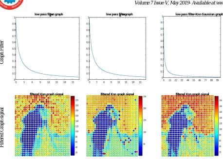
[image:6.595.216.358.546.698.2]Figure 8.shows the Gaussian kernel Graph signal of the original image and figure 7 (first row, left to right) shows graph signal of noisy image after adding original image with speckle noise, salt & pepper noise and Gaussian noise respectively, (second row, left to right) shows low pass filter constructed for respective graph signal shown in the first row and (third row, left to right) shows filtered graph signal of respective noise image in the first row. From figure 7 and figure 9 it can be understood that de-noising the image by low pass filtering of the kNN graph signal is better than the Gaussian kernel graph for all three type of noise that we considered here.
Fig.8.Gaussian Graph Signal
filtered Knn graph signal
20 40 60 80 100 120 140 160 180 200 filtered Knn graph signal
50 100 150 200 250 filtered Knn graph signal
20 40 60 80 100 120 140 160 180 200 220
0 11 22 33 44 55 66 77 88 99 0 0.1 0.2 0.3 0.4 0.5 0.6 0.7 0.8 0.9
1 low pass filter-Knn Gaussian graph
0 3 6 9 12 15 18 21
0 0.1 0.2 0.3 0.4 0.5 0.6 0.7 0.8 0.9 1
low pass filterKnn graph
0 3 6 9 12 15 18 21
0 0.1 0.2 0.3 0.4 0.5 0.6 0.7 0.8 0.9 1
Speckle noise Salt &Pepper noise Gaussian noise
G
ra
p
h
S
ig
n
al
w
it
h
n
o
is
e
G
ra
p
h
F
il
te
r
F
il
te
re
d
G
ra
p
h
s
ig
n
al
Fig.9. Gaussian kernal Graph performance for noise signal
V. CONCLUSIONS
In this paper, we analyzed the effect various methods of graph construction for the image processing using the graphical signal processing techniques, specifically using filtering operation on the noisy image. The e-ball graph construction method has the problem of selecting the right threshold value for ball radius suitable to the image without having the knowledge on the image perior to processing. Region graph construction method is suitable for segmention problem as it perform more smoothing of the image by forming the super pixels. The Gaussian kernel graph is not reflecting the connectivity of the underlying structure of the image as it shows gap between the eigen value. From the analysis it can be understood that the knn graph construction method is more suitable for processing the image using future promising graph signal processing. This is more evident in the application of graph filtering operation to the different types of the noise added images. To strengthen the identification of the right graph construction method to be used for image processing ,various application like compression, recognition can be tried.
REFERENCES
[1] DI Shuman, SK Narang, P Frossard "The emerging field of signal processing on graphs: Extending high-dimensional data analysis to networks and other irregular domains” IEEE Signal Processing Magazine, 2013
[3] T. Jebara, J. Wang, S. Chang, "Graph Construction and B-Matching for Semi-Supervised Learning", Proc. Int'l Conf. Machine Learning, pp. 441-448, 2009.
[4] W Dong, C Moses, K Li“Efficient k-nearest neighbor graph construction for generic similarity measures” International World Wide Web Conference Committee
(IW3C2),2011.
[5] KHajebi, YAbbasi-Yadkori,HShahbazi “Fast approximate nearest-neighbor search with k-nearest neighbor graph” Proceedings of the Twenty-Second International
Joint Conference on Artificial Intelligence, 2011 .
[6] Xiao L., Dai B., Fang Y., Wu T. (2012) Kernel L1 Graph for Image Analysis. In: Liu CL., Zhang C., Wang L. (eds) Pattern Recognition. CCPR 2012.
Communications in Computer and Information Science, vol 321. Springer.
[7] T Gärtner, K Driessens, J Ramon “Graph kernels and gaussian processes for relational reinforcement” Machine learning, 2006,64:91–119 DOI
10.1007/s10994-006-8258-y.
[8] D. Romero, M. Ma, G. B. Giannakis, "Kernel-based reconstruction of graph signals", IEEE Trans. Signal Process., vol. 65, no. 3, pp. 764-778, Feb. 2017.
[9] J. Bégaint, D. Thoreau, P. Guillotel and C. Guillemot, "Region-Based Prediction for Image Compression in the Cloud," in IEEE Transactions on Image Processing,
vol. 27, no. 4, pp. 1835-1846,
[10] A. Sandryhaila, J. M. F. Moura, "Discrete signal processing on graphs", IEEE Trans. Signal Process., vol. 61, no. 7, pp. 1644-1656, Apr. 2013.
[11] G Fracastoro, D Thanou, P Frossard“Graph-based Transform Coding with Application to Image Compression“ in arxiv preprint arxiv:1712.06393, 2017.
[12] S. Chen, A. Sandryhaila, J. M. F. Moura and J. Kovacevic, "Signal denoising on graphs via graph filtering," 2014 IEEE Global Conference on Signal and Information Processing (GlobalSIP), Atlanta, GA, 2014, pp. 872-876.
[13] Nicolas Tremblay , Paulo Gon¸calves , Pierre Borgnat” Design of graph filters and filterbanks” in arXiv:1711.02046v1 [eess.SP] 3 Nov 2017
[14] N Perraudin, J Paratte, D Shuman, L Martin “GSPBOX: A toolbox for signal processing on graphs” inarxiv preprint arXiv , 2014
[15] Steven Kay, Butler “Eigenvalues and structures of graphs” a thesis university of california, san diego in 2008.
[16] Andries E. Brouwer, Willem H. Haemers “Spectra of graphs” published bySpringer-Verlag New York, 2012